Stacking layers

Do not see them differently

Do not consider all as the same

Unwaveringly, practice guarding the One

In Geographic Information Systems 🌐, geographic data is arranged as different ‘layers’ 🍰. For example:

• Multispectral or hyperspectral 🌈 optical satellites collect different radiometric bands from slices along the electromagnetic spectrum

• Synthetic Aperture Radar (SAR) 📡 sensors have different polarizations such as HH, HV, VH & VV

• Satellite laser and radar altimeters 🛰️ measure elevation which can be turned into a Digital Elevation Model (DEM)

As long as these layers are georeferenced 📍 though, they can be stacked! This tutorial will cover the following topics:

• Searching for spatiotemporal datasets in a dynamic STAC Catalog 📚

• Stacking time-series 📆 data into a 4D tensor of shape (time, channel, y, x)

• Organizing different geographic 🗺️ layers into a dataset suitable for change detection

🎉 Getting started

Load up them libraries!

import os

import matplotlib.pyplot as plt
import numpy as np
import planetary_computer
import pystac
import rasterio
import torch
import torchdata
import xarray as xr
import zen3geo

0️⃣ Search for spatiotemporal data 📅

This time, we’ll be looking at change detection using time-series data. The focus area is Gunung Talamau, Sumatra Barat, Indonesia 🇮🇩 where an earthquake on 25 Feb 2022 triggered a series of landslides ⛰️. Affected areas will be mapped using Sentinel-1 Radiometrically Terrain Corrected (RTC) intensity SAR data 📡 obtained via a spatiotemporal query to a STAC API.

🔗 Links:

• UNOSAT satellite-detected landslide maps over Pasaman, Indonesia

• Humanitarian Data Exchange link

• Microsoft Planetary Computer STAC Explorer

This is how the Sentinel-1 radar image looks like over Sumatra Barat, Indonesia on 23 February 2022, two days before the earthquake.

Sentinel-1 PolSAR time-series ⏳

Before we start, we’ll need to set the PC_SDK_SUBSCRIPTION_KEY environment variable 🔡 to access the Sentinel-1 RTC data from Planetary Computer 💻. The steps are:

1. Get a 🪐 Planetary Computer account at https://planetarycomputer.microsoft.com/account/request

2. Follow 🧑‍🏫 instructions to get a subscription key

3. Go to https://planetarycomputer.developer.azure-api.net/profile. You should have a Primary key 🔑 and Secondary key 🗝️, click on ‘Show’ to reveal it. Copy and paste the key below, or better, set it securely 🔐 in something like a.env file!

# Uncomment the line below and set your Planetary Computer subscription key
# os.environ["PC_SDK_SUBSCRIPTION_KEY"] = "abcdefghijklmnopqrstuvwxyz123456"

Done? Let’s now define an 🧭 area of interest and 📆 time range covering one month before and one month after the earthquake ⚠️.

# Spatiotemporal query on STAC catalog for Sentinel-1 RTC data
query = dict(
    bbox=[99.8, -0.24, 100.07, 0.15],  # West, South, East, North
    datetime=["2022-01-25T00:00:00Z", "2022-03-25T23:59:59Z"],
    collections=["sentinel-1-rtc"],
)
dp = torchdata.datapipes.iter.IterableWrapper(iterable=[query])

Then, search over a dynamic STAC Catalog 📚 for items matching the spatiotemporal query ❔ using zen3geo.datapipes.PySTACAPISearcher (functional name: search_for_pystac_item).

dp_pystac_client = dp.search_for_pystac_item(
    catalog_url="https://planetarycomputer.microsoft.com/api/stac/v1",
    modifier=planetary_computer.sign_inplace,
)

Tip

Confused about which parameters go where 😕? Here’s some clarification:

1. Different spatiotemporal queries (e.g. for multiple geographical areas) should go in torchdata.datapipes.iter.IterableWrapper, e.g. IterableWrapper(iterable=[query_area1, query_area2]). The query dictionaries will be passed to pystac_client.Client.search().

2. Common parameters to interact with the STAC API Client should go in search_for_pystac_item(), e.g. the STAC API’s URL (see https://stacindex.org/catalogs?access=public&type=api for a public list) and connection related parameters. These will be passed to pystac_client.Client.open().

The output is a pystac_client.ItemSearch 🔎 instance that only holds the STAC API query information ℹ️ but doesn’t request for data! We’ll need to order it 🧞 to return something like a pystac.ItemCollection.

def get_all_items(item_search) -> pystac.ItemCollection:
    return item_search.item_collection()

dp_sen1_items = dp_pystac_client.map(fn=get_all_items)
dp_sen1_items

MapperIterDataPipe

Take a peek 🫣 to see if the query does contain STAC items.

it = iter(dp_sen1_items)
item_collection = next(it)
item_collection.items

[<Item id=S1A_IW_GRDH_1SDV_20220320T230514_20220320T230548_042411_050E99_rtc>,
 <Item id=S1A_IW_GRDH_1SDV_20220320T230449_20220320T230514_042411_050E99_rtc>,
 <Item id=S1A_IW_GRDH_1SDV_20220319T114141_20220319T114206_042389_050DD7_rtc>,
 <Item id=S1A_IW_GRDH_1SDV_20220308T230513_20220308T230548_042236_0508AF_rtc>,
 <Item id=S1A_IW_GRDH_1SDV_20220308T230448_20220308T230513_042236_0508AF_rtc>,
 <Item id=S1A_IW_GRDH_1SDV_20220307T114141_20220307T114206_042214_0507E8_rtc>,
 <Item id=S1A_IW_GRDH_1SDV_20220224T230514_20220224T230548_042061_0502B9_rtc>,
 <Item id=S1A_IW_GRDH_1SDV_20220224T230449_20220224T230514_042061_0502B9_rtc>,
 <Item id=S1A_IW_GRDH_1SDV_20220223T114141_20220223T114206_042039_0501F9_rtc>,
 <Item id=S1A_IW_GRDH_1SDV_20220212T230514_20220212T230548_041886_04FCA5_rtc>,
 <Item id=S1A_IW_GRDH_1SDV_20220212T230449_20220212T230514_041886_04FCA5_rtc>,
 <Item id=S1A_IW_GRDH_1SDV_20220211T114141_20220211T114206_041864_04FBD9_rtc>,
 <Item id=S1A_IW_GRDH_1SDV_20220131T230514_20220131T230548_041711_04F691_rtc>,
 <Item id=S1A_IW_GRDH_1SDV_20220131T230449_20220131T230514_041711_04F691_rtc>,
 <Item id=S1A_IW_GRDH_1SDV_20220130T114142_20220130T114207_041689_04F5D0_rtc>]

Copernicus Digital Elevation Model (DEM) ⛰️

Since landslides 🛝 typically happen on steep slopes, it can be useful to have a 🏔️ topographic layer. Let’s set up a STAC query 🙋 to get the 30m spatial resolution Copernicus DEM.

# Spatiotemporal query on STAC catalog for Copernicus DEM 30m data
query = dict(
    bbox=[99.8, -0.24, 100.07, 0.15],  # West, South, East, North
    collections=["cop-dem-glo-30"],
)
dp_copdem30 = torchdata.datapipes.iter.IterableWrapper(iterable=[query])

Just to be fancy, let’s chain 🔗 together the next two datapipes.

dp_copdem30_items = dp_copdem30.search_for_pystac_item(
    catalog_url="https://planetarycomputer.microsoft.com/api/stac/v1",
    modifier=planetary_computer.sign_inplace,
).map(fn=get_all_items)
dp_copdem30_items

MapperIterDataPipe

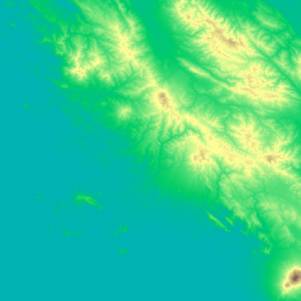
This is one of the four DEM tiles 🀫 that will be returned from the query.

Landslide extent vector polygons 🔶

Now for the target labels 🏷️. Following Vector segmentation masks, we’ll first load the digitized landslide polygons from a vector file 📁 using zen3geo.datapipes.PyogrioReader (functional name: read_from_pyogrio).

# https://gdal.org/user/virtual_file_systems.html#vsizip-zip-archives
shape_url = "/vsizip/vsicurl/https://unosat-maps.web.cern.ch/ID/LS20220308IDN/LS20220308IDN_SHP.zip/LS20220308IDN_SHP/S2_20220304_LandslideExtent_MountTalakmau.shp"

dp_shapes = torchdata.datapipes.iter.IterableWrapper(iterable=[shape_url])
dp_pyogrio = dp_shapes.read_from_pyogrio()
dp_pyogrio

PyogrioReaderIterDataPipe

Let’s take a look at the geopandas.GeoDataFrame data table 📊 to see the attributes inside.

it = iter(dp_pyogrio)
geodataframe = next(it)
print(geodataframe.bounds)
geodataframe.dropna(axis="columns")

        minx      miny        maxx      maxy
0  99.806331 -0.248744  100.065765  0.147054

	SensorDate	EventCode	Area_m2	Area_ha	Shape_Leng	Shape_Area	SensorID	Confidence	FieldValid	Main_Dmg	StaffID	geometry
0	2022-04-03	LS20220308IDN	6238480.0	623.848	2.873971	0.000507	Sentinel-2	To Be Evaluated	Not yet field validated	Landslide	TH	MULTIPOLYGON (((99.80642 -0.24865, 99.80642 -0...

We’ll show you what the landslide segmentation masks 😷 look like after it’s been rasterized later 😉.

1️⃣ Stack bands, append variables 📚

There are now three layers 🍰 to handle, two rasters and a vector. This section will show you step by step 📶 instructions to combine them using xarray like so:

1. Stack the Sentinel-1 🛰️ time-series STAC Items (GeoTIFFs) into an xarray.DataArray.

2. Combine the Sentinel-1 and Copernicus DEM ⛰️ xarray.DataArray layers into a single xarray.Dataset.

3. Using the xarray.Dataset as a canvas template, rasterize the landslide 🛝 polygon extents, and append the resulting segmentation mask as another data variable 🗃️ in the xarray.Dataset.

Stack multi-channel time-series GeoTIFFs 🗓️

Each pystac.Item in a pystac.ItemCollection represents a 🛰️ Sentinel-1 RTC image captured at a particular datetime ⌚. Let’s subset the data to just the mountain area, and stack 🥞 all the STAC items into a 4D time-series tensor using zen3geo.datapipes.StackSTACStacker (functional name: stack_stac_items)!

dp_sen1_stack = dp_sen1_items.stack_stac_items(
    assets=["vh", "vv"],  # SAR polarizations
    epsg=32647,  # UTM Zone 47N
    resolution=30,  # Spatial resolution of 30 metres
    bounds_latlon=[99.933681, -0.009951, 100.065765, 0.147054], # W, S, E, N
    xy_coords="center",  # pixel centroid coords instead of topleft corner
    dtype=np.float16,  # Use a lightweight data type
)
dp_sen1_stack

StackSTACStackerIterDataPipe

The keyword arguments are 📨 passed to stackstac.stack() behind the scenes. The important❕parameters to set in this case are:

• assets: The STAC item assets 🍱 (typically the ‘band’ names)

• epsg: The 🌐 EPSG projection code, best if you know the native projection

• resolution: Spatial resolution 📏. The Sentinel-1 RTC is actually at 10m, but we’ll resample to 30m to keep things small 🤏 and match the Copernicus DEM.

The result is a single xarray.DataArray ‘datacube’ 🧊 with dimensions (time, band, y, x).

it = iter(dp_sen1_stack)
dataarray = next(it)
dataarray

<xarray.DataArray 'stackstac-3b069ee52dbc03b1fd6c981837d6c185' (time: 15,
                                                                band: 2,
                                                                y: 579, x: 491)>
dask.array<fetch_raster_window, shape=(15, 2, 579, 491), dtype=float16, chunksize=(1, 1, 579, 491), chunktype=numpy.ndarray>
Coordinates: (12/39)
  * time                                   (time) datetime64[ns] 2022-01-30T1...
    id                                     (time) <U66 'S1A_IW_GRDH_1SDV_2022...
  * band                                   (band) <U2 'vh' 'vv'
  * x                                      (x) float64 6.039e+05 ... 6.186e+05
  * y                                      (y) float64 1.624e+04 ... -1.095e+03
    sar:resolution_range                   int64 20
    ...                                     ...
    sar:looks_equivalent_number            float64 4.4
    sat:absolute_orbit                     (time) int64 41689 41711 ... 42411
    description                            (band) <U173 'Terrain-corrected ga...
    title                                  (band) <U41 'VH: vertical transmit...
    raster:bands                           object {'nodata': -32768, 'data_ty...
    epsg                                   int64 32647
Attributes:
    spec:        RasterSpec(epsg=32647, bounds=(603870, -1110, 618600, 16260)...
    crs:         epsg:32647
    transform:   | 30.00, 0.00, 603870.00|\n| 0.00,-30.00, 16260.00|\n| 0.00,...
    resolution:  30

xarray.DataArray

'stackstac-3b069ee52dbc03b1fd6c981837d6c185'

• time: 15
• band: 2
• y: 579
• x: 491

• dask.array<chunksize=(1, 1, 579, 491), meta=np.ndarray>

  Array Chunk Bytes 16.27 MiB 555.25 kiB Shape (15, 2, 579, 491) (1, 1, 579, 491) Count 3 Graph Layers 30 Chunks Type float16 numpy.ndarray

• Coordinates: (39)
  • time
    (time)
    datetime64[ns]
    2022-01-30T11:41:54.579841 ... 2...

    array(['2022-01-30T11:41:54.579841000', '2022-01-31T23:05:01.682395000',
           '2022-01-31T23:05:31.361312000', '2022-02-11T11:41:54.431563000',
           '2022-02-12T23:05:01.659360000', '2022-02-12T23:05:31.338948000',
           '2022-02-23T11:41:54.329096000', '2022-02-24T23:05:01.545399000',
           '2022-02-24T23:05:31.225720000', '2022-03-07T11:41:54.128217000',
           '2022-03-08T23:05:01.372152000', '2022-03-08T23:05:31.049372000',
           '2022-03-19T11:41:54.298948000', '2022-03-20T23:05:01.651958000',
           '2022-03-20T23:05:31.322477000'], dtype='datetime64[ns]')

  • id
    (time)
    <U66
    'S1A_IW_GRDH_1SDV_20220130T11414...

    array(['S1A_IW_GRDH_1SDV_20220130T114142_20220130T114207_041689_04F5D0_rtc',
           'S1A_IW_GRDH_1SDV_20220131T230449_20220131T230514_041711_04F691_rtc',
           'S1A_IW_GRDH_1SDV_20220131T230514_20220131T230548_041711_04F691_rtc',
           'S1A_IW_GRDH_1SDV_20220211T114141_20220211T114206_041864_04FBD9_rtc',
           'S1A_IW_GRDH_1SDV_20220212T230449_20220212T230514_041886_04FCA5_rtc',
           'S1A_IW_GRDH_1SDV_20220212T230514_20220212T230548_041886_04FCA5_rtc',
           'S1A_IW_GRDH_1SDV_20220223T114141_20220223T114206_042039_0501F9_rtc',
           'S1A_IW_GRDH_1SDV_20220224T230449_20220224T230514_042061_0502B9_rtc',
           'S1A_IW_GRDH_1SDV_20220224T230514_20220224T230548_042061_0502B9_rtc',
           'S1A_IW_GRDH_1SDV_20220307T114141_20220307T114206_042214_0507E8_rtc',
           'S1A_IW_GRDH_1SDV_20220308T230448_20220308T230513_042236_0508AF_rtc',
           'S1A_IW_GRDH_1SDV_20220308T230513_20220308T230548_042236_0508AF_rtc',
           'S1A_IW_GRDH_1SDV_20220319T114141_20220319T114206_042389_050DD7_rtc',
           'S1A_IW_GRDH_1SDV_20220320T230449_20220320T230514_042411_050E99_rtc',
           'S1A_IW_GRDH_1SDV_20220320T230514_20220320T230548_042411_050E99_rtc'],
          dtype='<U66')

  • band
    (band)
    <U2
    'vh' 'vv'

    array(['vh', 'vv'], dtype='<U2')

  • x
    (x)
    float64
    6.039e+05 6.039e+05 ... 6.186e+05

    array([603885., 603915., 603945., ..., 618525., 618555., 618585.])

  • y
    (y)
    float64
    1.624e+04 1.622e+04 ... -1.095e+03

    array([16245., 16215., 16185., ..., -1035., -1065., -1095.])

  • sar:resolution_range
    ()
    int64
    20

    array(20)

  • sar:looks_range
    ()
    int64
    5

    array(5)

  • s1:processing_level
    ()
    <U1
    '1'

    array('1', dtype='<U1')

  • platform
    ()
    <U11
    'SENTINEL-1A'

    array('SENTINEL-1A', dtype='<U11')

  • sar:looks_azimuth
    ()
    int64
    1

    array(1)

  • sar:polarizations
    ()
    object
    {'VH', 'VV'}

    array({'VH', 'VV'}, dtype=object)

  • s1:datatake_id
    (time)
    <U6
    '325072' '325265' ... '331417'

    array(['325072', '325265', '325265', '326617', '326821', '326821',
           '328185', '328377', '328377', '329704', '329903', '329903',
           '331223', '331417', '331417'], dtype='<U6')

  • sar:pixel_spacing_azimuth
    ()
    int64
    10

    array(10)

  • end_datetime
    (time)
    <U32
    '2022-01-30 11:42:07.078874+00:0...

    array(['2022-01-30 11:42:07.078874+00:00',
           '2022-01-31 23:05:14.181446+00:00',
           '2022-01-31 23:05:48.539689+00:00',
           '2022-02-11 11:42:06.930653+00:00',
           '2022-02-12 23:05:14.158379+00:00',
           '2022-02-12 23:05:48.518027+00:00',
           '2022-02-23 11:42:06.828173+00:00',
           '2022-02-24 23:05:14.044423+00:00',
           '2022-02-24 23:05:48.405549+00:00',
           '2022-03-07 11:42:06.627352+00:00',
           '2022-03-08 23:05:13.871115+00:00',
           '2022-03-08 23:05:48.226141+00:00',
           '2022-03-19 11:42:06.798097+00:00',
           '2022-03-20 23:05:14.150921+00:00',
           '2022-03-20 23:05:48.492544+00:00'], dtype='<U32')

  • sar:instrument_mode
    ()
    <U2
    'IW'

    array('IW', dtype='<U2')

  • s1:product_timeliness
    ()
    <U8
    'Fast-24h'

    array('Fast-24h', dtype='<U8')

  • s1:total_slices
    (time)
    <U2
    '9' '15' '15' '9' ... '9' '15' '15'

    array(['9', '15', '15', '9', '15', '15', '9', '15', '15', '9', '15', '15',
           '9', '15', '15'], dtype='<U2')

  • s1:instrument_configuration_ID
    ()
    <U1
    '7'

    array('7', dtype='<U1')

  • sar:pixel_spacing_range
    ()
    int64
    10

    array(10)

  • sat:orbit_state
    (time)
    <U10
    'ascending' ... 'descending'

    array(['ascending', 'descending', 'descending', 'ascending', 'descending',
           'descending', 'ascending', 'descending', 'descending', 'ascending',
           'descending', 'descending', 'ascending', 'descending',
           'descending'], dtype='<U10')

  • sat:platform_international_designator
    ()
    <U9
    '2014-016A'

    array('2014-016A', dtype='<U9')

  • sat:relative_orbit
    (time)
    int64
    142 164 164 142 ... 164 142 164 164

    array([142, 164, 164, 142, 164, 164, 142, 164, 164, 142, 164, 164, 142,
           164, 164])

  • sar:center_frequency
    ()
    float64
    5.405

    array(5.405)

  • sar:observation_direction
    ()
    <U5
    'right'

    array('right', dtype='<U5')

  • sar:frequency_band
    ()
    <U1
    'C'

    array('C', dtype='<U1')

  • s1:orbit_source
    (time)
    <U6
    'PREORB' 'RESORB' ... 'RESORB'

    array(['PREORB', 'RESORB', 'RESORB', 'PREORB', 'RESORB', 'RESORB',
           'PREORB', 'RESORB', 'RESORB', 'PREORB', 'RESORB', 'RESORB',
           'PREORB', 'RESORB', 'RESORB'], dtype='<U6')

  • sar:resolution_azimuth
    ()
    int64
    22

    array(22)

  • s1:resolution
    ()
    <U4
    'high'

    array('high', dtype='<U4')

  • start_datetime
    (time)
    <U32
    '2022-01-30 11:41:42.080807+00:0...

    array(['2022-01-30 11:41:42.080807+00:00',
           '2022-01-31 23:04:49.183345+00:00',
           '2022-01-31 23:05:14.182935+00:00',
           '2022-02-11 11:41:41.932473+00:00',
           '2022-02-12 23:04:49.160340+00:00',
           '2022-02-12 23:05:14.159868+00:00',
           '2022-02-23 11:41:41.830019+00:00',
           '2022-02-24 23:04:49.046375+00:00',
           '2022-02-24 23:05:14.045892+00:00',
           '2022-03-07 11:41:41.629081+00:00',
           '2022-03-08 23:04:48.873188+00:00',
           '2022-03-08 23:05:13.872604+00:00',
           '2022-03-19 11:41:41.799800+00:00',
           '2022-03-20 23:04:49.152996+00:00',
           '2022-03-20 23:05:14.152410+00:00'], dtype='<U32')

  • constellation
    ()
    <U10
    'Sentinel-1'

    array('Sentinel-1', dtype='<U10')

  • proj:epsg
    ()
    int64
    32647

    array(32647)

  • s1:slice_number
    (time)
    <U2
    '3' '14' '15' '3' ... '3' '14' '15'

    array(['3', '14', '15', '3', '14', '15', '3', '14', '15', '3', '14', '15',
           '3', '14', '15'], dtype='<U2')

  • sar:product_type
    ()
    <U3
    'GRD'

    array('GRD', dtype='<U3')

  • sar:looks_equivalent_number
    ()
    float64
    4.4

    array(4.4)

  • sat:absolute_orbit
    (time)
    int64
    41689 41711 41711 ... 42411 42411

    array([41689, 41711, 41711, 41864, 41886, 41886, 42039, 42061, 42061,
           42214, 42236, 42236, 42389, 42411, 42411])

  • description
    (band)
    <U173
    'Terrain-corrected gamma naught ...

    array(['Terrain-corrected gamma naught values of signal transmitted with vertical polarization and received with horizontal polarization with radiometric terrain correction applied.',
           'Terrain-corrected gamma naught values of signal transmitted with vertical polarization and received with vertical polarization with radiometric terrain correction applied.'],
          dtype='<U173')

  • title
    (band)
    <U41
    'VH: vertical transmit, horizont...

    array(['VH: vertical transmit, horizontal receive',
           'VV: vertical transmit, vertical receive'], dtype='<U41')

  • raster:bands
    ()
    object
    {'nodata': -32768, 'data_type': ...

    array({'nodata': -32768, 'data_type': 'float32', 'spatial_resolution': 10.0},
          dtype=object)

  • epsg
    ()
    int64
    32647

    array(32647)

• Attributes: (4)

  spec :

  RasterSpec(epsg=32647, bounds=(603870, -1110, 618600, 16260), resolutions_xy=(30, 30))

  crs :

  epsg:32647

  transform :

  | 30.00, 0.00, 603870.00| | 0.00,-30.00, 16260.00| | 0.00, 0.00, 1.00|

  resolution :

  30

Append single-band DEM to datacube 🧊

Time for layer number 2 💕. Let’s read the Copernicus DEM ⛰️ STAC Item into an xarray.DataArray first, again via zen3geo.datapipes.StackSTACStacker (functional name: stack_stac_items). We’ll need to ensure ✔️ that the DEM is reprojected to the same 🌏 coordinate reference system and 📐 aligned to the same spatial extent as the Sentinel-1 time-series.

dp_copdem_stack = dp_copdem30_items.stack_stac_items(
    assets=["data"],
    epsg=32647,  # UTM Zone 47N
    resolution=30,  # Spatial resolution of 30 metres
    bounds_latlon=[99.933681, -0.009951, 100.065765, 0.147054], # W, S, E, N
    xy_coords="center",  # pixel centroid coords instead of topleft corner
    dtype=np.float16,  # Use a lightweight data type
    resampling=rasterio.enums.Resampling.bilinear,  # Bilinear resampling
)
dp_copdem_stack

StackSTACStackerIterDataPipe

it = iter(dp_copdem_stack)
dataarray = next(it)
dataarray

<xarray.DataArray 'stackstac-afdc91bccb12ec4ba1376f87b0641b62' (time: 4,
                                                                band: 1,
                                                                y: 579, x: 491)>
dask.array<fetch_raster_window, shape=(4, 1, 579, 491), dtype=float16, chunksize=(1, 1, 579, 491), chunktype=numpy.ndarray>
Coordinates:
  * time        (time) datetime64[ns] 2021-04-22 2021-04-22 ... 2021-04-22
    id          (time) <U40 'Copernicus_DSM_COG_10_S01_00_E100_00_DEM' ... 'C...
  * band        (band) <U4 'data'
  * x           (x) float64 6.039e+05 6.039e+05 ... 6.186e+05 6.186e+05
  * y           (y) float64 1.624e+04 1.622e+04 ... -1.065e+03 -1.095e+03
    proj:epsg   int64 4326
    platform    <U8 'TanDEM-X'
    gsd         int64 30
    proj:shape  object {3600}
    epsg        int64 32647
Attributes:
    spec:        RasterSpec(epsg=32647, bounds=(603870, -1110, 618600, 16260)...
    crs:         epsg:32647
    transform:   | 30.00, 0.00, 603870.00|\n| 0.00,-30.00, 16260.00|\n| 0.00,...
    resolution:  30

xarray.DataArray

'stackstac-afdc91bccb12ec4ba1376f87b0641b62'

• time: 4
• band: 1
• y: 579
• x: 491

• dask.array<chunksize=(1, 1, 579, 491), meta=np.ndarray>

  Array Chunk Bytes 2.17 MiB 555.25 kiB Shape (4, 1, 579, 491) (1, 1, 579, 491) Count 3 Graph Layers 4 Chunks Type float16 numpy.ndarray

• Coordinates: (10)
  • time
    (time)
    datetime64[ns]
    2021-04-22 ... 2021-04-22

    array(['2021-04-22T00:00:00.000000000', '2021-04-22T00:00:00.000000000',
           '2021-04-22T00:00:00.000000000', '2021-04-22T00:00:00.000000000'],
          dtype='datetime64[ns]')

  • id
    (time)
    <U40
    'Copernicus_DSM_COG_10_S01_00_E1...

    array(['Copernicus_DSM_COG_10_S01_00_E100_00_DEM',
           'Copernicus_DSM_COG_10_S01_00_E099_00_DEM',
           'Copernicus_DSM_COG_10_N00_00_E100_00_DEM',
           'Copernicus_DSM_COG_10_N00_00_E099_00_DEM'], dtype='<U40')

  • band
    (band)
    <U4
    'data'

    array(['data'], dtype='<U4')

  • x
    (x)
    float64
    6.039e+05 6.039e+05 ... 6.186e+05

    array([603885., 603915., 603945., ..., 618525., 618555., 618585.])

  • y
    (y)
    float64
    1.624e+04 1.622e+04 ... -1.095e+03

    array([16245., 16215., 16185., ..., -1035., -1065., -1095.])

  • proj:epsg
    ()
    int64
    4326

    array(4326)

  • platform
    ()
    <U8
    'TanDEM-X'

    array('TanDEM-X', dtype='<U8')

  • gsd
    ()
    int64
    30

    array(30)

  • proj:shape
    ()
    object
    {3600}

    array({3600}, dtype=object)

  • epsg
    ()
    int64
    32647

    array(32647)

• Attributes: (4)

  spec :

  RasterSpec(epsg=32647, bounds=(603870, -1110, 618600, 16260), resolutions_xy=(30, 30))

  crs :

  epsg:32647

  transform :

  | 30.00, 0.00, 603870.00| | 0.00,-30.00, 16260.00| | 0.00, 0.00, 1.00|

  resolution :

  30

Why are there 4 ⏳ time layers? Actually, the STAC query had returned four DEM tiles 🀫, and stackstac.stack() has stacked both of them along a dimension name ‘time’ (probably better named ‘tile’). Fear not, the tiles can be joined 🍒 into a single terrain mosaic layer with dimensions (“band”, “y”, “x”) using zen3geo.datapipes.StackSTACMosaicker (functional name: mosaic_dataarray).

dp_copdem_mosaic = dp_copdem_stack.mosaic_dataarray(nodata=0)
dp_copdem_mosaic

StackSTACMosaickerIterDataPipe

Great! The two xarray.DataArray objects (Sentinel-1 and Copernicus DEM mosaic) can now be combined 🪢. First, use torchdata.datapipes.iter.Zipper (functional name: zip) to put the two xarray.DataArray objects into a tuple 🎵.

dp_sen1_copdem = dp_sen1_stack.zip(dp_copdem_mosaic)
dp_sen1_copdem

ZipperIterDataPipe

Next, use torchdata.datapipes.iter.Collator (functional name: collate) to convert 🤸 the tuple of xarray.DataArray objects into an xarray.Dataset 🧊, similar to what was done in Object detection boxes.

def sardem_collate_fn(sar_and_dem: tuple) -> xr.Dataset:
    """
    Combine a pair of xarray.DataArray (SAR, DEM) inputs into an
    xarray.Dataset with data variables named 'vh', 'vv' and 'dem'.
    """
    # Turn 2 xr.DataArray objects into 1 xr.Dataset with multiple data vars
    sar, dem = sar_and_dem

    # Initialize xr.Dataset with VH and VV channels
    dataset: xr.Dataset = sar.sel(band="vh").to_dataset(name="vh")
    dataset["vv"] = sar.sel(band="vv")

    # Add Copernicus DEM mosaic as another layer
    dataset["dem"] = dem.squeeze()

    return dataset

dp_vhvvdem_dataset = dp_sen1_copdem.collate(collate_fn=sardem_collate_fn)
dp_vhvvdem_dataset

CollatorIterDataPipe

Here’s how the current xarray.Dataset 🧱 is structured. Notice that VH and VV polarization channels 📡 are now two separate data variables, each with dimensions (time, y, x). The DEM ⛰️ data is not a time-series, so it has dimensions (y, x) only. All the ‘band’ dimensions have been removed ❌ and are now data variables within the xarray.Dataset 😎.

it = iter(dp_vhvvdem_dataset)
dataset = next(it)
dataset

<xarray.Dataset>
Dimensions:                                (time: 15, x: 491, y: 579)
Coordinates: (12/41)
  * time                                   (time) datetime64[ns] 2022-01-30T1...
    id                                     (time) <U66 'S1A_IW_GRDH_1SDV_2022...
    band                                   <U2 'vh'
  * x                                      (x) float64 6.039e+05 ... 6.186e+05
  * y                                      (y) float64 1.624e+04 ... -1.095e+03
    sar:resolution_range                   int64 20
    ...                                     ...
    description                            <U173 'Terrain-corrected gamma nau...
    title                                  <U41 'VH: vertical transmit, horiz...
    raster:bands                           object {'nodata': -32768, 'data_ty...
    epsg                                   int64 32647
    gsd                                    int64 30
    proj:shape                             object {3600}
Data variables:
    vh                                     (time, y, x) float16 dask.array<chunksize=(1, 579, 491), meta=np.ndarray>
    vv                                     (time, y, x) float16 dask.array<chunksize=(1, 579, 491), meta=np.ndarray>
    dem                                    (y, x) float16 dask.array<chunksize=(579, 491), meta=np.ndarray>

xarray.Dataset

• Dimensions:
  • time: 15
  • x: 491
  • y: 579
• Coordinates: (41)
  • time
    (time)
    datetime64[ns]
    2022-01-30T11:41:54.579841 ... 2...

    array(['2022-01-30T11:41:54.579841000', '2022-01-31T23:05:01.682395000',
           '2022-01-31T23:05:31.361312000', '2022-02-11T11:41:54.431563000',
           '2022-02-12T23:05:01.659360000', '2022-02-12T23:05:31.338948000',
           '2022-02-23T11:41:54.329096000', '2022-02-24T23:05:01.545399000',
           '2022-02-24T23:05:31.225720000', '2022-03-07T11:41:54.128217000',
           '2022-03-08T23:05:01.372152000', '2022-03-08T23:05:31.049372000',
           '2022-03-19T11:41:54.298948000', '2022-03-20T23:05:01.651958000',
           '2022-03-20T23:05:31.322477000'], dtype='datetime64[ns]')

  • id
    (time)
    <U66
    'S1A_IW_GRDH_1SDV_20220130T11414...

    array(['S1A_IW_GRDH_1SDV_20220130T114142_20220130T114207_041689_04F5D0_rtc',
           'S1A_IW_GRDH_1SDV_20220131T230449_20220131T230514_041711_04F691_rtc',
           'S1A_IW_GRDH_1SDV_20220131T230514_20220131T230548_041711_04F691_rtc',
           'S1A_IW_GRDH_1SDV_20220211T114141_20220211T114206_041864_04FBD9_rtc',
           'S1A_IW_GRDH_1SDV_20220212T230449_20220212T230514_041886_04FCA5_rtc',
           'S1A_IW_GRDH_1SDV_20220212T230514_20220212T230548_041886_04FCA5_rtc',
           'S1A_IW_GRDH_1SDV_20220223T114141_20220223T114206_042039_0501F9_rtc',
           'S1A_IW_GRDH_1SDV_20220224T230449_20220224T230514_042061_0502B9_rtc',
           'S1A_IW_GRDH_1SDV_20220224T230514_20220224T230548_042061_0502B9_rtc',
           'S1A_IW_GRDH_1SDV_20220307T114141_20220307T114206_042214_0507E8_rtc',
           'S1A_IW_GRDH_1SDV_20220308T230448_20220308T230513_042236_0508AF_rtc',
           'S1A_IW_GRDH_1SDV_20220308T230513_20220308T230548_042236_0508AF_rtc',
           'S1A_IW_GRDH_1SDV_20220319T114141_20220319T114206_042389_050DD7_rtc',
           'S1A_IW_GRDH_1SDV_20220320T230449_20220320T230514_042411_050E99_rtc',
           'S1A_IW_GRDH_1SDV_20220320T230514_20220320T230548_042411_050E99_rtc'],
          dtype='<U66')

  • band
    ()
    <U2
    'vh'

    array('vh', dtype='<U2')

  • x
    (x)
    float64
    6.039e+05 6.039e+05 ... 6.186e+05

    array([603885., 603915., 603945., ..., 618525., 618555., 618585.])

  • y
    (y)
    float64
    1.624e+04 1.622e+04 ... -1.095e+03

    array([16245., 16215., 16185., ..., -1035., -1065., -1095.])

  • sar:resolution_range
    ()
    int64
    20

    array(20)

  • sar:looks_range
    ()
    int64
    5

    array(5)

  • s1:processing_level
    ()
    <U1
    '1'

    array('1', dtype='<U1')

  • platform
    ()
    <U11
    'SENTINEL-1A'

    array('SENTINEL-1A', dtype='<U11')

  • sar:looks_azimuth
    ()
    int64
    1

    array(1)

  • sar:polarizations
    ()
    object
    {'VH', 'VV'}

    array({'VH', 'VV'}, dtype=object)

  • s1:datatake_id
    (time)
    <U6
    '325072' '325265' ... '331417'

    array(['325072', '325265', '325265', '326617', '326821', '326821',
           '328185', '328377', '328377', '329704', '329903', '329903',
           '331223', '331417', '331417'], dtype='<U6')

  • sar:pixel_spacing_azimuth
    ()
    int64
    10

    array(10)

  • end_datetime
    (time)
    <U32
    '2022-01-30 11:42:07.078874+00:0...

    array(['2022-01-30 11:42:07.078874+00:00',
           '2022-01-31 23:05:14.181446+00:00',
           '2022-01-31 23:05:48.539689+00:00',
           '2022-02-11 11:42:06.930653+00:00',
           '2022-02-12 23:05:14.158379+00:00',
           '2022-02-12 23:05:48.518027+00:00',
           '2022-02-23 11:42:06.828173+00:00',
           '2022-02-24 23:05:14.044423+00:00',
           '2022-02-24 23:05:48.405549+00:00',
           '2022-03-07 11:42:06.627352+00:00',
           '2022-03-08 23:05:13.871115+00:00',
           '2022-03-08 23:05:48.226141+00:00',
           '2022-03-19 11:42:06.798097+00:00',
           '2022-03-20 23:05:14.150921+00:00',
           '2022-03-20 23:05:48.492544+00:00'], dtype='<U32')

  • sar:instrument_mode
    ()
    <U2
    'IW'

    array('IW', dtype='<U2')

  • s1:product_timeliness
    ()
    <U8
    'Fast-24h'

    array('Fast-24h', dtype='<U8')

  • s1:total_slices
    (time)
    <U2
    '9' '15' '15' '9' ... '9' '15' '15'

    array(['9', '15', '15', '9', '15', '15', '9', '15', '15', '9', '15', '15',
           '9', '15', '15'], dtype='<U2')

  • s1:instrument_configuration_ID
    ()
    <U1
    '7'

    array('7', dtype='<U1')

  • sar:pixel_spacing_range
    ()
    int64
    10

    array(10)

  • sat:orbit_state
    (time)
    <U10
    'ascending' ... 'descending'

    array(['ascending', 'descending', 'descending', 'ascending', 'descending',
           'descending', 'ascending', 'descending', 'descending', 'ascending',
           'descending', 'descending', 'ascending', 'descending',
           'descending'], dtype='<U10')

  • sat:platform_international_designator
    ()
    <U9
    '2014-016A'

    array('2014-016A', dtype='<U9')

  • sat:relative_orbit
    (time)
    int64
    142 164 164 142 ... 164 142 164 164

    array([142, 164, 164, 142, 164, 164, 142, 164, 164, 142, 164, 164, 142,
           164, 164])

  • sar:center_frequency
    ()
    float64
    5.405

    array(5.405)

  • sar:observation_direction
    ()
    <U5
    'right'

    array('right', dtype='<U5')

  • sar:frequency_band
    ()
    <U1
    'C'

    array('C', dtype='<U1')

  • s1:orbit_source
    (time)
    <U6
    'PREORB' 'RESORB' ... 'RESORB'

    array(['PREORB', 'RESORB', 'RESORB', 'PREORB', 'RESORB', 'RESORB',
           'PREORB', 'RESORB', 'RESORB', 'PREORB', 'RESORB', 'RESORB',
           'PREORB', 'RESORB', 'RESORB'], dtype='<U6')

  • sar:resolution_azimuth
    ()
    int64
    22

    array(22)

  • s1:resolution
    ()
    <U4
    'high'

    array('high', dtype='<U4')

  • start_datetime
    (time)
    <U32
    '2022-01-30 11:41:42.080807+00:0...

    array(['2022-01-30 11:41:42.080807+00:00',
           '2022-01-31 23:04:49.183345+00:00',
           '2022-01-31 23:05:14.182935+00:00',
           '2022-02-11 11:41:41.932473+00:00',
           '2022-02-12 23:04:49.160340+00:00',
           '2022-02-12 23:05:14.159868+00:00',
           '2022-02-23 11:41:41.830019+00:00',
           '2022-02-24 23:04:49.046375+00:00',
           '2022-02-24 23:05:14.045892+00:00',
           '2022-03-07 11:41:41.629081+00:00',
           '2022-03-08 23:04:48.873188+00:00',
           '2022-03-08 23:05:13.872604+00:00',
           '2022-03-19 11:41:41.799800+00:00',
           '2022-03-20 23:04:49.152996+00:00',
           '2022-03-20 23:05:14.152410+00:00'], dtype='<U32')

  • constellation
    ()
    <U10
    'Sentinel-1'

    array('Sentinel-1', dtype='<U10')

  • proj:epsg
    ()
    int64
    32647

    array(32647)

  • s1:slice_number
    (time)
    <U2
    '3' '14' '15' '3' ... '3' '14' '15'

    array(['3', '14', '15', '3', '14', '15', '3', '14', '15', '3', '14', '15',
           '3', '14', '15'], dtype='<U2')

  • sar:product_type
    ()
    <U3
    'GRD'

    array('GRD', dtype='<U3')

  • sar:looks_equivalent_number
    ()
    float64
    4.4

    array(4.4)

  • sat:absolute_orbit
    (time)
    int64
    41689 41711 41711 ... 42411 42411

    array([41689, 41711, 41711, 41864, 41886, 41886, 42039, 42061, 42061,
           42214, 42236, 42236, 42389, 42411, 42411])

  • description
    ()
    <U173
    'Terrain-corrected gamma naught ...

    array('Terrain-corrected gamma naught values of signal transmitted with vertical polarization and received with horizontal polarization with radiometric terrain correction applied.',
          dtype='<U173')

  • title
    ()
    <U41
    'VH: vertical transmit, horizont...

    array('VH: vertical transmit, horizontal receive', dtype='<U41')

  • raster:bands
    ()
    object
    {'nodata': -32768, 'data_type': ...

    array({'nodata': -32768, 'data_type': 'float32', 'spatial_resolution': 10.0},
          dtype=object)

  • epsg
    ()
    int64
    32647

    array(32647)

  • gsd
    ()
    int64
    30

    array(30)

  • proj:shape
    ()
    object
    {3600}

    array({3600}, dtype=object)

• Data variables: (3)
  • vh
    (time, y, x)
    float16
    dask.array<chunksize=(1, 579, 491), meta=np.ndarray>

    spec :

    RasterSpec(epsg=32647, bounds=(603870, -1110, 618600, 16260), resolutions_xy=(30, 30))

    crs :

    epsg:32647

    transform :

    | 30.00, 0.00, 603870.00| | 0.00,-30.00, 16260.00| | 0.00, 0.00, 1.00|

    resolution :

    30

    Array Chunk Bytes 8.13 MiB 555.25 kiB Shape (15, 579, 491) (1, 579, 491) Count 4 Graph Layers 15 Chunks Type float16 numpy.ndarray

  • vv
    (time, y, x)
    float16
    dask.array<chunksize=(1, 579, 491), meta=np.ndarray>

    spec :

    RasterSpec(epsg=32647, bounds=(603870, -1110, 618600, 16260), resolutions_xy=(30, 30))

    crs :

    epsg:32647

    transform :

    | 30.00, 0.00, 603870.00| | 0.00,-30.00, 16260.00| | 0.00, 0.00, 1.00|

    resolution :

    30

    Array Chunk Bytes 8.13 MiB 555.25 kiB Shape (15, 579, 491) (1, 579, 491) Count 4 Graph Layers 15 Chunks Type float16 numpy.ndarray

  • dem
    (y, x)
    float16
    dask.array<chunksize=(579, 491), meta=np.ndarray>

    spec :

    RasterSpec(epsg=32647, bounds=(603870, -1110, 618600, 16260), resolutions_xy=(30, 30))

    crs :

    epsg:32647

    transform :

    | 30.00, 0.00, 603870.00| | 0.00,-30.00, 16260.00| | 0.00, 0.00, 1.00|

    resolution :

    30

    Array Chunk Bytes 555.25 kiB 555.25 kiB Shape (579, 491) (579, 491) Count 6 Graph Layers 1 Chunks Type float16 numpy.ndarray

• Attributes: (0)

Visualize the DataPipe graph ⛓️ too for good measure.

torchdata.datapipes.utils.to_graph(dp=dp_vhvvdem_dataset)

Rasterize target labels to datacube extent 🏷️

The landslide polygons 🔶 can now be rasterized and added as another layer to our datacube 🧊. Following Vector segmentation masks, we’ll first fork the DataPipe into two branches 🫒 using torchdata.datapipes.iter.Forker (functional name: fork).

dp_vhvvdem_canvas, dp_vhvvdem_datacube = dp_vhvvdem_dataset.fork(num_instances=2)
dp_vhvvdem_canvas, dp_vhvvdem_datacube

(_ChildDataPipe, _ChildDataPipe)

Next, create a blank canvas 📃 using zen3geo.datapipes.XarrayCanvas (functional name: canvas_from_xarray) and rasterize 🖌 the vector polygons onto the template canvas using zen3geo.datapipes.DatashaderRasterizer (functional name: rasterize_with_datashader)

dp_datashader = dp_vhvvdem_canvas.canvas_from_xarray().rasterize_with_datashader(
    vector_datapipe=dp_pyogrio
)
dp_datashader

DatashaderRasterizerIterDataPipe

Cool, and this layer can be added 🧮 as another data variable in the datacube.

def cubemask_collate_fn(cube_and_mask: tuple) -> xr.Dataset:
    """
    Merge target 'mask' (xarray.DataArray) into an existing datacube
    (xarray.Dataset) as another data variable.
    """
    datacube, mask = cube_and_mask

    merged_datacube = xr.merge(objects=[datacube, mask.rename("mask")], join="override")

    return merged_datacube

dp_datacube = dp_vhvvdem_datacube.zip(dp_datashader).collate(
    collate_fn=cubemask_collate_fn
)
dp_datacube

CollatorIterDataPipe

Inspect the datacube 🧊 and visualize all the layers 🧅 within.

it = iter(dp_datacube)
datacube = next(it)
datacube

<xarray.Dataset>
Dimensions:                                (time: 15, x: 491, y: 579)
Coordinates: (12/42)
  * time                                   (time) datetime64[ns] 2022-01-30T1...
    id                                     (time) <U66 'S1A_IW_GRDH_1SDV_2022...
    band                                   <U2 'vh'
  * x                                      (x) float64 6.039e+05 ... 6.186e+05
  * y                                      (y) float64 1.624e+04 ... -1.095e+03
    sar:resolution_range                   int64 20
    ...                                     ...
    title                                  <U41 'VH: vertical transmit, horiz...
    raster:bands                           object {'nodata': -32768, 'data_ty...
    epsg                                   int64 32647
    gsd                                    int64 30
    proj:shape                             object {3600}
    spatial_ref                            int64 0
Data variables:
    vh                                     (time, y, x) float16 dask.array<chunksize=(1, 579, 491), meta=np.ndarray>
    vv                                     (time, y, x) float16 dask.array<chunksize=(1, 579, 491), meta=np.ndarray>
    dem                                    (y, x) float16 dask.array<chunksize=(579, 491), meta=np.ndarray>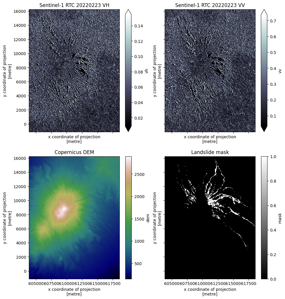
    mask                                   (y, x) uint8 0 0 0 0 0 ... 0 0 0 0 0

xarray.Dataset

• Dimensions:
  • time: 15
  • x: 491
  • y: 579
• Coordinates: (42)
  • time
    (time)
    datetime64[ns]
    2022-01-30T11:41:54.579841 ... 2...

    array(['2022-01-30T11:41:54.579841000', '2022-01-31T23:05:01.682395000',
           '2022-01-31T23:05:31.361312000', '2022-02-11T11:41:54.431563000',
           '2022-02-12T23:05:01.659360000', '2022-02-12T23:05:31.338948000',
           '2022-02-23T11:41:54.329096000', '2022-02-24T23:05:01.545399000',
           '2022-02-24T23:05:31.225720000', '2022-03-07T11:41:54.128217000',
           '2022-03-08T23:05:01.372152000', '2022-03-08T23:05:31.049372000',
           '2022-03-19T11:41:54.298948000', '2022-03-20T23:05:01.651958000',
           '2022-03-20T23:05:31.322477000'], dtype='datetime64[ns]')

  • id
    (time)
    <U66
    'S1A_IW_GRDH_1SDV_20220130T11414...

    array(['S1A_IW_GRDH_1SDV_20220130T114142_20220130T114207_041689_04F5D0_rtc',
           'S1A_IW_GRDH_1SDV_20220131T230449_20220131T230514_041711_04F691_rtc',
           'S1A_IW_GRDH_1SDV_20220131T230514_20220131T230548_041711_04F691_rtc',
           'S1A_IW_GRDH_1SDV_20220211T114141_20220211T114206_041864_04FBD9_rtc',
           'S1A_IW_GRDH_1SDV_20220212T230449_20220212T230514_041886_04FCA5_rtc',
           'S1A_IW_GRDH_1SDV_20220212T230514_20220212T230548_041886_04FCA5_rtc',
           'S1A_IW_GRDH_1SDV_20220223T114141_20220223T114206_042039_0501F9_rtc',
           'S1A_IW_GRDH_1SDV_20220224T230449_20220224T230514_042061_0502B9_rtc',
           'S1A_IW_GRDH_1SDV_20220224T230514_20220224T230548_042061_0502B9_rtc',
           'S1A_IW_GRDH_1SDV_20220307T114141_20220307T114206_042214_0507E8_rtc',
           'S1A_IW_GRDH_1SDV_20220308T230448_20220308T230513_042236_0508AF_rtc',
           'S1A_IW_GRDH_1SDV_20220308T230513_20220308T230548_042236_0508AF_rtc',
           'S1A_IW_GRDH_1SDV_20220319T114141_20220319T114206_042389_050DD7_rtc',
           'S1A_IW_GRDH_1SDV_20220320T230449_20220320T230514_042411_050E99_rtc',
           'S1A_IW_GRDH_1SDV_20220320T230514_20220320T230548_042411_050E99_rtc'],
          dtype='<U66')

  • band
    ()
    <U2
    'vh'

    array('vh', dtype='<U2')

  • x
    (x)
    float64
    6.039e+05 6.039e+05 ... 6.186e+05

    axis :

    X

    long_name :

    x coordinate of projection

    standard_name :

    projection_x_coordinate

    units :

    metre

    array([603885., 603915., 603945., ..., 618525., 618555., 618585.])

  • y
    (y)
    float64
    1.624e+04 1.622e+04 ... -1.095e+03

    axis :

    Y

    long_name :

    y coordinate of projection

    standard_name :

    projection_y_coordinate

    units :

    metre

    array([16245., 16215., 16185., ..., -1035., -1065., -1095.])

  • sar:resolution_range
    ()
    int64
    20

    array(20)

  • sar:looks_range
    ()
    int64
    5

    array(5)

  • s1:processing_level
    ()
    <U1
    '1'

    array('1', dtype='<U1')

  • platform
    ()
    <U11
    'SENTINEL-1A'

    array('SENTINEL-1A', dtype='<U11')

  • sar:looks_azimuth
    ()
    int64
    1

    array(1)

  • sar:polarizations
    ()
    object
    {'VH', 'VV'}

    array({'VH', 'VV'}, dtype=object)

  • s1:datatake_id
    (time)
    <U6
    '325072' '325265' ... '331417'

    array(['325072', '325265', '325265', '326617', '326821', '326821',
           '328185', '328377', '328377', '329704', '329903', '329903',
           '331223', '331417', '331417'], dtype='<U6')

  • sar:pixel_spacing_azimuth
    ()
    int64
    10

    array(10)

  • end_datetime
    (time)
    <U32
    '2022-01-30 11:42:07.078874+00:0...

    array(['2022-01-30 11:42:07.078874+00:00',
           '2022-01-31 23:05:14.181446+00:00',
           '2022-01-31 23:05:48.539689+00:00',
           '2022-02-11 11:42:06.930653+00:00',
           '2022-02-12 23:05:14.158379+00:00',
           '2022-02-12 23:05:48.518027+00:00',
           '2022-02-23 11:42:06.828173+00:00',
           '2022-02-24 23:05:14.044423+00:00',
           '2022-02-24 23:05:48.405549+00:00',
           '2022-03-07 11:42:06.627352+00:00',
           '2022-03-08 23:05:13.871115+00:00',
           '2022-03-08 23:05:48.226141+00:00',
           '2022-03-19 11:42:06.798097+00:00',
           '2022-03-20 23:05:14.150921+00:00',
           '2022-03-20 23:05:48.492544+00:00'], dtype='<U32')

  • sar:instrument_mode
    ()
    <U2
    'IW'

    array('IW', dtype='<U2')

  • s1:product_timeliness
    ()
    <U8
    'Fast-24h'

    array('Fast-24h', dtype='<U8')

  • s1:total_slices
    (time)
    <U2
    '9' '15' '15' '9' ... '9' '15' '15'

    array(['9', '15', '15', '9', '15', '15', '9', '15', '15', '9', '15', '15',
           '9', '15', '15'], dtype='<U2')

  • s1:instrument_configuration_ID
    ()
    <U1
    '7'

    array('7', dtype='<U1')

  • sar:pixel_spacing_range
    ()
    int64
    10

    array(10)

  • sat:orbit_state
    (time)
    <U10
    'ascending' ... 'descending'

    array(['ascending', 'descending', 'descending', 'ascending', 'descending',
           'descending', 'ascending', 'descending', 'descending', 'ascending',
           'descending', 'descending', 'ascending', 'descending',
           'descending'], dtype='<U10')

  • sat:platform_international_designator
    ()
    <U9
    '2014-016A'

    array('2014-016A', dtype='<U9')

  • sat:relative_orbit
    (time)
    int64
    142 164 164 142 ... 164 142 164 164

    array([142, 164, 164, 142, 164, 164, 142, 164, 164, 142, 164, 164, 142,
           164, 164])

  • sar:center_frequency
    ()
    float64
    5.405

    array(5.405)

  • sar:observation_direction
    ()
    <U5
    'right'

    array('right', dtype='<U5')

  • sar:frequency_band
    ()
    <U1
    'C'

    array('C', dtype='<U1')

  • s1:orbit_source
    (time)
    <U6
    'PREORB' 'RESORB' ... 'RESORB'

    array(['PREORB', 'RESORB', 'RESORB', 'PREORB', 'RESORB', 'RESORB',
           'PREORB', 'RESORB', 'RESORB', 'PREORB', 'RESORB', 'RESORB',
           'PREORB', 'RESORB', 'RESORB'], dtype='<U6')

  • sar:resolution_azimuth
    ()
    int64
    22

    array(22)

  • s1:resolution
    ()
    <U4
    'high'

    array('high', dtype='<U4')

  • start_datetime
    (time)
    <U32
    '2022-01-30 11:41:42.080807+00:0...

    array(['2022-01-30 11:41:42.080807+00:00',
           '2022-01-31 23:04:49.183345+00:00',
           '2022-01-31 23:05:14.182935+00:00',
           '2022-02-11 11:41:41.932473+00:00',
           '2022-02-12 23:04:49.160340+00:00',
           '2022-02-12 23:05:14.159868+00:00',
           '2022-02-23 11:41:41.830019+00:00',
           '2022-02-24 23:04:49.046375+00:00',
           '2022-02-24 23:05:14.045892+00:00',
           '2022-03-07 11:41:41.629081+00:00',
           '2022-03-08 23:04:48.873188+00:00',
           '2022-03-08 23:05:13.872604+00:00',
           '2022-03-19 11:41:41.799800+00:00',
           '2022-03-20 23:04:49.152996+00:00',
           '2022-03-20 23:05:14.152410+00:00'], dtype='<U32')

  • constellation
    ()
    <U10
    'Sentinel-1'

    array('Sentinel-1', dtype='<U10')

  • proj:epsg
    ()
    int64
    32647

    array(32647)

  • s1:slice_number
    (time)
    <U2
    '3' '14' '15' '3' ... '3' '14' '15'

    array(['3', '14', '15', '3', '14', '15', '3', '14', '15', '3', '14', '15',
           '3', '14', '15'], dtype='<U2')

  • sar:product_type
    ()
    <U3
    'GRD'

    array('GRD', dtype='<U3')

  • sar:looks_equivalent_number
    ()
    float64
    4.4

    array(4.4)

  • sat:absolute_orbit
    (time)
    int64
    41689 41711 41711 ... 42411 42411

    array([41689, 41711, 41711, 41864, 41886, 41886, 42039, 42061, 42061,
           42214, 42236, 42236, 42389, 42411, 42411])

  • description
    ()
    <U173
    'Terrain-corrected gamma naught ...

    array('Terrain-corrected gamma naught values of signal transmitted with vertical polarization and received with horizontal polarization with radiometric terrain correction applied.',
          dtype='<U173')

  • title
    ()
    <U41
    'VH: vertical transmit, horizont...

    array('VH: vertical transmit, horizontal receive', dtype='<U41')

  • raster:bands
    ()
    object
    {'nodata': -32768, 'data_type': ...

    array({'nodata': -32768, 'data_type': 'float32', 'spatial_resolution': 10.0},
          dtype=object)

  • epsg
    ()
    int64
    32647

    array(32647)

  • gsd
    ()
    int64
    30

    array(30)

  • proj:shape
    ()
    object
    {3600}

    array({3600}, dtype=object)

  • spatial_ref
    ()
    int64
    0

    crs_wkt :

    PROJCS["WGS 84 / UTM zone 47N",GEOGCS["WGS 84",DATUM["WGS_1984",SPHEROID["WGS 84",6378137,298.257223563,AUTHORITY["EPSG","7030"]],AUTHORITY["EPSG","6326"]],PRIMEM["Greenwich",0,AUTHORITY["EPSG","8901"]],UNIT["degree",0.0174532925199433,AUTHORITY["EPSG","9122"]],AUTHORITY["EPSG","4326"]],PROJECTION["Transverse_Mercator"],PARAMETER["latitude_of_origin",0],PARAMETER["central_meridian",99],PARAMETER["scale_factor",0.9996],PARAMETER["false_easting",500000],PARAMETER["false_northing",0],UNIT["metre",1,AUTHORITY["EPSG","9001"]],AXIS["Easting",EAST],AXIS["Northing",NORTH],AUTHORITY["EPSG","32647"]]

    semi_major_axis :

    6378137.0

    semi_minor_axis :

    6356752.314245179

    inverse_flattening :

    298.257223563

    reference_ellipsoid_name :

    WGS 84

    longitude_of_prime_meridian :

    0.0

    prime_meridian_name :

    Greenwich

    geographic_crs_name :

    WGS 84

    horizontal_datum_name :

    World Geodetic System 1984

    projected_crs_name :

    WGS 84 / UTM zone 47N

    grid_mapping_name :

    transverse_mercator

    latitude_of_projection_origin :

    0.0

    longitude_of_central_meridian :

    99.0

    false_easting :

    500000.0

    false_northing :

    0.0

    scale_factor_at_central_meridian :

    0.9996

    spatial_ref :

    PROJCS["WGS 84 / UTM zone 47N",GEOGCS["WGS 84",DATUM["WGS_1984",SPHEROID["WGS 84",6378137,298.257223563,AUTHORITY["EPSG","7030"]],AUTHORITY["EPSG","6326"]],PRIMEM["Greenwich",0,AUTHORITY["EPSG","8901"]],UNIT["degree",0.0174532925199433,AUTHORITY["EPSG","9122"]],AUTHORITY["EPSG","4326"]],PROJECTION["Transverse_Mercator"],PARAMETER["latitude_of_origin",0],PARAMETER["central_meridian",99],PARAMETER["scale_factor",0.9996],PARAMETER["false_easting",500000],PARAMETER["false_northing",0],UNIT["metre",1,AUTHORITY["EPSG","9001"]],AXIS["Easting",EAST],AXIS["Northing",NORTH],AUTHORITY["EPSG","32647"]]

    GeoTransform :

    603870.0 30.000000000000004 0.0 16260.0 0.0 -30.000000000000004

    array(0)

• Data variables: (4)
  • vh
    (time, y, x)
    float16
    dask.array<chunksize=(1, 579, 491), meta=np.ndarray>

    spec :

    RasterSpec(epsg=32647, bounds=(603870, -1110, 618600, 16260), resolutions_xy=(30, 30))

    crs :

    epsg:32647

    transform :

    | 30.00, 0.00, 603870.00| | 0.00,-30.00, 16260.00| | 0.00, 0.00, 1.00|

    resolution :

    30

    Array Chunk Bytes 8.13 MiB 555.25 kiB Shape (15, 579, 491) (1, 579, 491) Count 4 Graph Layers 15 Chunks Type float16 numpy.ndarray

  • vv
    (time, y, x)
    float16
    dask.array<chunksize=(1, 579, 491), meta=np.ndarray>

    spec :

    RasterSpec(epsg=32647, bounds=(603870, -1110, 618600, 16260), resolutions_xy=(30, 30))

    crs :

    epsg:32647

    transform :

    | 30.00, 0.00, 603870.00| | 0.00,-30.00, 16260.00| | 0.00, 0.00, 1.00|

    resolution :

    30

    Array Chunk Bytes 8.13 MiB 555.25 kiB Shape (15, 579, 491) (1, 579, 491) Count 4 Graph Layers 15 Chunks Type float16 numpy.ndarray

  • dem
    (y, x)
    float16
    dask.array<chunksize=(579, 491), meta=np.ndarray>

    spec :

    RasterSpec(epsg=32647, bounds=(603870, -1110, 618600, 16260), resolutions_xy=(30, 30))

    crs :

    epsg:32647

    transform :

    | 30.00, 0.00, 603870.00| | 0.00,-30.00, 16260.00| | 0.00, 0.00, 1.00|

    resolution :

    30

    Array Chunk Bytes 555.25 kiB 555.25 kiB Shape (579, 491) (579, 491) Count 6 Graph Layers 1 Chunks Type float16 numpy.ndarray

  • mask
    (y, x)
    uint8
    0 0 0 0 0 0 0 0 ... 0 0 0 0 0 0 0 0

    _FillValue :

    255

    array([[0, 0, 0, ..., 0, 0, 0],
           [0, 0, 0, ..., 0, 0, 0],
           [0, 0, 0, ..., 0, 0, 0],
           ...,
           [0, 0, 0, ..., 0, 0, 0],
           [0, 0, 0, ..., 0, 0, 0],
           [0, 0, 0, ..., 0, 0, 0]], dtype=uint8)

• Attributes: (0)

dataslice = datacube.sel(time="2022-02-23T11:41:54.329096000").compute()

fig, ax = plt.subplots(nrows=2, ncols=2, figsize=(11, 12), sharex=True, sharey=True)

dataslice.vh.plot.imshow(ax=ax[0][0], cmap="bone", robust=True)
ax[0][0].set_title("Sentinel-1 RTC 20220223 VH")

dataslice.vv.plot.imshow(ax=ax[0][1], cmap="bone", robust=True)
ax[0][1].set_title("Sentinel-1 RTC 20220223 VV")

dataslice.dem.plot.imshow(ax=ax[1][0], cmap="gist_earth")
ax[1][0].set_title("Copernicus DEM")

dataslice.mask.plot.imshow(ax=ax[1][1], cmap="binary_r")
ax[1][1].set_title("Landslide mask")

plt.show()

2️⃣ Splitters and lumpers 🪨

There are many ways to do change detection 🕵️. Here is but one ☝️.

Slice spatially and temporally 💇

For the splitters, let’s first slice the datacube along the spatial dimension into 256x256 chips 🍪 using zen3geo.datapipes.XbatcherSlicer (functional name: slice_with_xbatcher). Refer to Chipping and batching data if you need a 🧑‍🎓 refresher.

dp_xbatcher = dp_datacube.slice_with_xbatcher(input_dims={"y": 256, "x": 256})
dp_xbatcher

XbatcherSlicerIterDataPipe

Next, we’ll use the earthquake ⚠️ date to divide each 256x256 SAR time-series chip 🍕 with dimensions (time, y, x) into pre-event and post-event tensors. The target landslide 🛝 mask will be split out too.

def pre_post_target_tuple(
    datachip: xr.Dataset, event_time: str = "2022-02-25T01:39:27"
) -> tuple[xr.Dataset, xr.Dataset, xr.Dataset]:
    """
    From a single xarray.Dataset, split it into a tuple containing the
    pre/post/target tensors.
    """
    pre_times = datachip.time <= np.datetime64(event_time)
    post_times = datachip.time > np.datetime64(event_time)

    return (
        datachip.sel(time=pre_times)[["vv", "vh", "dem"]],
        datachip.sel(time=post_times)[["vv", "vh", "dem"]],
        datachip[["mask"]],
    )

dp_pre_post_target = dp_xbatcher.map(fn=pre_post_target_tuple)
dp_pre_post_target

MapperIterDataPipe

Inspect 👀 the shapes of one of the data chips that has been split into pre/post/target 🍡 xarray.Dataset objects.

it = iter(dp_pre_post_target)
pre, post, target = next(it)
print(f"Before: {pre.sizes}")
print(f"After: {post.sizes}")
print(f"Target: {target.sizes}")

/home/docs/checkouts/readthedocs.org/user_builds/zen3geo/envs/v0.5.0/lib/python3.10/site-packages/torch/utils/data/datapipes/iter/combining.py:248: UserWarning: Some child DataPipes are not exhausted when __iter__ is called. We are resetting the buffer and each child DataPipe will read from the start again.
  warnings.warn("Some child DataPipes are not exhausted when __iter__ is called. We are resetting "

Before: Frozen({'time': 9, 'y': 256, 'x': 256})
After: Frozen({'time': 6, 'y': 256, 'x': 256})
Target: Frozen({'y': 256, 'x': 256})

Cool, at this point, you may want to decide 🤔 on how to handle different sized before and after time-series images 🎞️. Or maybe not, and torch.Tensor objects are all you desire ❤️‍🔥.

def dataset_to_tensors(triple_tuple) -> (torch.Tensor, torch.Tensor, torch.Tensor):
    """
    Converts xarray.Datasets in a tuple into torch.Tensor objects.
    """
    pre, post, target = triple_tuple

    _pre: torch.Tensor = torch.as_tensor(pre.to_array().data)
    _post: torch.Tensor = torch.as_tensor(post.to_array().data)
    _target: torch.Tensor = torch.as_tensor(target.mask.data.astype("uint8"))

    return _pre, _post, _target

dp_tensors = dp_pre_post_target.map(fn=dataset_to_tensors)
dp_tensors

MapperIterDataPipe

This is the final DataPipe graph ⛓️.

torchdata.datapipes.utils.to_graph(dp=dp_tensors)

Into a DataLoader 🏋️

Time to connect the DataPipe to torch.utils.data.DataLoader ♻️!

dataloader = torch.utils.data.DataLoader2(dataset=dp_tensors, batch_size=None)
for i, batch in enumerate(dataloader):
    pre, post, target = batch
    print(f"Batch {i} - pre: {pre.shape}, post: {post.shape}, target: {target.shape}")

/home/docs/checkouts/readthedocs.org/user_builds/zen3geo/envs/v0.5.0/lib/python3.10/site-packages/torch/utils/data/datapipes/iter/combining.py:248: UserWarning: Some child DataPipes are not exhausted when __iter__ is called. We are resetting the buffer and each child DataPipe will read from the start again.
  warnings.warn("Some child DataPipes are not exhausted when __iter__ is called. We are resetting "

Batch 0 - pre: torch.Size([3, 9, 256, 256]), post: torch.Size([3, 6, 256, 256]), target: torch.Size([256, 256])
Batch 1 - pre: torch.Size([3, 9, 256, 256]), post: torch.Size([3, 6, 256, 256]), target: torch.Size([256, 256])

Don’t just see change, be the change 🪧!

See also

This data pipeline is adapted from (a subset of) some amazing 🧪 research done during the Frontier Development Lab 2022 - Self Supervised Learning on SAR data for Change Detection challenge 🚀. Watch the final showcase video at https://www.youtube.com/watch?v=igAUTJwbmsY 📽️!