Multi-resolution

Multi-resolution#

On top of a hundred foot pole you linger

Clinging to the first mark of the scale

How do you proceed higher?

It will take more than a leap of faith

Earth Observation 🛰️ and climate projection 🌡️ data can be captured at different levels of detail. In this lesson, we’ll work with a multitude of spatial resolutions 📏, learning to respect the ground sampling distance or native resolution 🔬 of the physical variable being measured, while 🪶 minimizing memory usage. By the end of the lesson, you should be able to:

Find 🔍 low and high spatial resolution climate datasets and load them from Zarr stores
Stack 🥞 and subset time-series datasets with different spatial resolutions stored in a hierarchical datatree.DataTree structure
Slice 🔪 the multi-resolution dataset along the time-axis into monthly bins

🔗 Links:

🎉 Getting started#

These are the tools 🛠️ you’ll need.

import matplotlib.pyplot as plt
import pandas as pd
import torchdata.dataloader2
import xarray as xr
import xpystac
import zen3geo

from datatree import DataTree

0️⃣ Find climate model datasets 🪸#

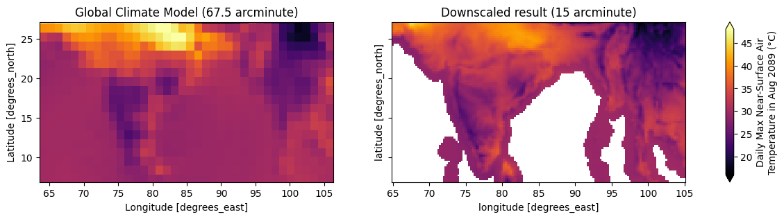
The two datasets we’ll be working with are 🌐 gridded climate projections, one that is in its original low 🔅 spatial resolution, and another one of a higher 🔆 spatial resolution. Specifically, we’ll be looking at the maximum temperature 🌡️ (tasmax) variable from one of the Coupled Model Intercomparison Project Phase 6 (CMIP6) global coupled ocean-atmosphere general circulation model (GCM) 💨 outputs that is of low-resolution (67.5 arcminute), and a super-resolution product from DeepSD 🤔 that is of a higher resolution (15 arcminute).

Note

The following tutorial will mostly use the term super-resolution 🔭 from Computer Vision instead of downscaling ⏬. It’s just that the term downscaling ⏬ (going from low to high resolution) can get confused with downsampling 🙃 (going from high to low resolution), whereas super-resolution 🔭 is unambiguously about going from low 🔅 to high 🔆 resolution.

🔖 References:

lowres_raw = "https://cpdataeuwest.blob.core.windows.net/cp-cmip/cmip6/ScenarioMIP/MRI/MRI-ESM2-0/ssp585/r1i1p1f1/Amon/tasmax/gn/v20191108"
highres_deepsd = "https://cpdataeuwest.blob.core.windows.net/cp-cmip/version1/data/DeepSD/ScenarioMIP.MRI.MRI-ESM2-0.ssp585.r1i1p1f1.month.DeepSD.tasmax.zarr"

This is how the projected maximum temperature 🥵 for August 2089 looks like over South Asia 🪷 for a low-resolution 🔅 Global Climate Model (left) and a high-resolution 🔆 downscaled product (right).

_images/ae6461c9172b93b138413387d3be026e2d36d193d15e1f2c770fe5a113fba459.png

Load Zarr stores 📦#

The Zarr stores 🧊 can be loaded into an xarray.Dataset via zen3geo.datapipes.XpySTACAssetReader (functional name: read_from_xpystac) with the engine="zarr" keyword argument.

dp_lowres = torchdata.datapipes.iter.IterableWrapper(iterable=[lowres_raw])
dp_highres = torchdata.datapipes.iter.IterableWrapper(iterable=[highres_deepsd])

dp_lowres_dataset = dp_lowres.read_from_xpystac(engine="zarr", chunks="auto")
dp_highres_dataset = dp_highres.read_from_xpystac(engine="zarr", chunks="auto")

Inspect the climate datasets 🔥#

Let’s now preview 👀 the low-resolution 🔅 and high-resolution 🔆 temperature datasets.

it = iter(dp_lowres_dataset)
ds_lowres = next(it)
ds_lowres

<xarray.Dataset> Size: 211MB
Dimensions:    (lat: 160, bnds: 2, lon: 320, time: 1032)
Coordinates:
    height     float64 8B ...
  * lat        (lat) float64 1kB -89.14 -88.03 -86.91 ... 86.91 88.03 89.14
    lat_bnds   (lat, bnds) float64 3kB dask.array<chunksize=(160, 2), meta=np.ndarray>
  * lon        (lon) float64 3kB 0.0 1.125 2.25 3.375 ... 356.6 357.8 358.9
    lon_bnds   (lon, bnds) float64 5kB dask.array<chunksize=(320, 2), meta=np.ndarray>
  * time       (time) datetime64[ns] 8kB 2015-01-16T12:00:00 ... 2100-12-16T1...
    time_bnds  (time, bnds) datetime64[ns] 17kB dask.array<chunksize=(1032, 2), meta=np.ndarray>
Dimensions without coordinates: bnds
Data variables:
    tasmax     (time, lat, lon) float32 211MB dask.array<chunksize=(516, 160, 320), meta=np.ndarray>
Attributes: (12/47)
    Conventions:            CF-1.7 CMIP-6.2
    activity_id:            ScenarioMIP
    branch_method:          standard
    branch_time_in_child:   60265.0
    branch_time_in_parent:  60265.0
    cmor_version:           3.4.0
    ...                     ...
    table_info:             Creation Date:(14 December 2018) MD5:b2d32d1a0d9b...
    title:                  MRI-ESM2-0 output prepared for CMIP6
    tracking_id:            hdl:21.14100/421f03b2-8cb7-4473-9d03-0f772c8969c4
    variable_id:            tasmax
    variant_label:          r1i1p1f1
    version_id:             v20191108

it = iter(dp_highres_dataset)
ds_highres = next(it)
ds_highres

<xarray.Dataset> Size: 4GB
Dimensions:  (lat: 720, lon: 1440, time: 1020)
Coordinates:
  * lat      (lat) float64 6kB -89.88 -89.62 -89.38 -89.12 ... 89.38 89.62 89.88
  * lon      (lon) float64 12kB -179.9 -179.6 -179.4 ... 179.4 179.6 179.9
  * time     (time) datetime64[ns] 8kB 2015-01-01 2015-02-01 ... 2099-12-01
Data variables:
    tasmax   (time, lat, lon) float32 4GB dask.array<chunksize=(1020, 144, 144), meta=np.ndarray>
Attributes: (12/17)
    Conventions:                     CF-1.8
    activity_id:                     ScenarioMIP
    cmip6_downscaling_contact:       hello@carbonplan.org
    cmip6_downscaling_explainer:     https://carbonplan.org/research/cmip6-do...
    cmip6_downscaling_institution:   CarbonPlan
    cmip6_downscaling_license:       CC-BY-4.0
    ...                              ...
    institution_id:                  MRI
    member_id:                       r1i1p1f1
    references:                      Eyring, V., Bony, S., Meehl, G. A., Seni...
    source_id:                       MRI-ESM2-0
    timescale:                       day
    variable_id:                     tasmax

Notice that the low-resolution 🔅 dataset has lon/lat pixels of shape (320, 160), whereas the high-resolution 🔆 dataset is of shape (1440, 720). So there has been a 4.5x increase 📈 in spatial resolution going from the raw GCM 🌐 grid to the super-resolution 🔭 DeepSD grid.

Shift from 0-360 to -180-180 🌐#

A sharp eye 👁️ would have noticed that the longitudinal range of the low-resolution 🔅 and high-resolution 🔆 dataset are offset ↔️ by 180°, going from 0° to 360° and -180° to +180° respectively. Let’s shift the coordinates 📍 of the low-resolution grid 🌍 from 0-360 to -180-180 using a custom torchdata.datapipes.iter.Mapper (functional name: map) function.

🔖 References:

def shift_longitude_360_to_180(ds: xr.Dataset) -> xr.Dataset:
    ds = ds.assign_coords(lon=(((ds.lon + 180) % 360) - 180))
    ds = ds.roll(lon=int(len(ds.lon) / 2), roll_coords=True)
    return ds

dp_lowres_dataset_180 = dp_lowres_dataset.map(fn=shift_longitude_360_to_180)
dp_lowres_dataset_180

MapperIterDataPipe

Double check that the low-resolution 🔆 grid’s longitude coordinates 🔢 are now in the -180° to +180° range.

it = iter(dp_lowres_dataset_180)
ds_lowres_180 = next(it)
ds_lowres_180

<xarray.Dataset> Size: 211MB
Dimensions:    (lat: 160, bnds: 2, lon: 320, time: 1032)
Coordinates:
    height     float64 8B ...
  * lat        (lat) float64 1kB -89.14 -88.03 -86.91 ... 86.91 88.03 89.14
    lat_bnds   (lat, bnds) float64 3kB dask.array<chunksize=(160, 2), meta=np.ndarray>
    lon_bnds   (lon, bnds) float64 5kB dask.array<chunksize=(320, 2), meta=np.ndarray>
  * time       (time) datetime64[ns] 8kB 2015-01-16T12:00:00 ... 2100-12-16T1...
    time_bnds  (time, bnds) datetime64[ns] 17kB dask.array<chunksize=(1032, 2), meta=np.ndarray>
  * lon        (lon) float64 3kB -180.0 -178.9 -177.8 ... 176.6 177.8 178.9
Dimensions without coordinates: bnds
Data variables:
    tasmax     (time, lat, lon) float32 211MB dask.array<chunksize=(516, 160, 320), meta=np.ndarray>
Attributes: (12/47)
    Conventions:            CF-1.7 CMIP-6.2
    activity_id:            ScenarioMIP
    branch_method:          standard
    branch_time_in_child:   60265.0
    branch_time_in_parent:  60265.0
    cmor_version:           3.4.0
    ...                     ...
    table_info:             Creation Date:(14 December 2018) MD5:b2d32d1a0d9b...
    title:                  MRI-ESM2-0 output prepared for CMIP6
    tracking_id:            hdl:21.14100/421f03b2-8cb7-4473-9d03-0f772c8969c4
    variable_id:            tasmax
    variant_label:          r1i1p1f1
    version_id:             v20191108

Spatiotemporal stack and subset 🍱#

Following on from Stacking layers where multiple 🥞 layers with the same spatial resolution were stacked together into an xarray.DataArray object, this section will teach 🧑‍🏫 you about stacking datasets with different spatial resolutions 📶 into a datatree.DataTree object that has a nested/hierarchical structure. That datatree.DataTree can then be subsetted 🥮 to the desired spatial and temporal extent in one go 😎.

Stack multi-resolution datasets 📚#

First, we’ll need to combine 🪢 the low-resolution GCM and high-resolution DeepSD xarray.Dataset objects into a tuple 🎵 using torchdata.datapipes.iter.Zipper (functional name: zip).

dp_lowres_highres = dp_lowres_dataset_180.zip(dp_highres_dataset)
dp_lowres_highres

ZipperIterDataPipe

Next, use torchdata.datapipes.iter.Collator (functional name: collate) to convert 🤸 the tuple of xarray.Dataset objects into an datatree.DataTree 🎋, similar to what was done in Stacking layers. Note that we’ll only take the ‘tasmax’ ♨️ (Daily Maximum Near-Surface Air Temperature) xarray.DataArray variable from each of the xarray.Dataset objects.

def multires_collate_fn(lowres_and_highres: tuple) -> DataTree:
    """
    Combine a pair of xarray.Dataset (lowres, highres) inputs into a
    datatree.DataTree with groups named 'lowres' and 'highres'.
    """
    # Turn 2 xr.Dataset objects into 1 xr.DataTree with multiple groups
    ds_lowres, ds_highres = lowres_and_highres

    # Create DataTree with lowres and highres groups
    datatree: DataTree = DataTree.from_dict(
        d={"lowres": ds_lowres.tasmax, "highres": ds_highres.tasmax}
    )

    return datatree

dp_datatree = dp_lowres_highres.collate(collate_fn=multires_collate_fn)
dp_datatree

CollatorIterDataPipe

See the nested 🪆 structure of the datatree.DataTree. The low-resolution 🔅 GCM and high-resolution 🔆 DeepSD outputs have been placed in separate groups 🖖.

it = iter(dp_datatree)
datatree = next(it)
datatree

<xarray.DatasetView> Size: 0B
Dimensions:  ()
Data variables:
    *empty*

Subset multi-resolution layers 🥮#

The climate model outputs above are a global 🗺️ one covering a timespan from January 2015 to December 2100 📅. If you’re only interested in a particular region 🌏 or timespan ⌚, then the datatree.DataTree will need to be trimmed 💇 down. Let’s use datatree.DataTree.sel() to subset the multi-resolution data to just the Philippines 🇵🇭 for the period 2015 to 2030.

def spatiotemporal_subset(dt: DataTree) -> DataTree:
    dt_subset = dt.sel(
        lon=slice(116.4375, 126.5625),
        lat=slice(5.607445, 19.065325),
        time=slice("2015-01-01", "2030-12-31"),
    )
    return dt_subset

dp_datatree_subset = dp_datatree.map(fn=spatiotemporal_subset)
dp_datatree_subset

MapperIterDataPipe

Inspect the subsetted climate dataset 🕵️

it = iter(dp_datatree_subset)
datatree_subset = next(it)
datatree_subset

<xarray.DatasetView> Size: 0B
Dimensions:  ()
Data variables: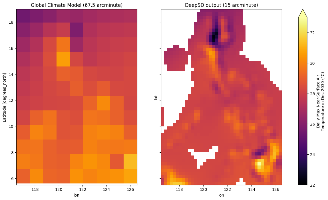
    *empty*

Let’s plot the projected temperature 🌡️ for Dec 2030 over the Philippine Archipelago to ensure things look ok.

ds_lowres = (
    datatree_subset["lowres/tasmax"]
    .sel(time=slice("2030-12-01", "2030-12-31"))
    .squeeze()
)
ds_lowres -= 273.15  # convert from Kelvin to Celsius
ds_highres = (
    datatree_subset["highres/tasmax"]
    .sel(time=slice("2030-12-01", "2030-12-31"))
    .squeeze()
)
ds_highres -= 273.15  # convert from Kelvin to Celsius

# Plot projected maximum temperature over the Philippines from GCM and DeepSD
fig, ax = plt.subplots(nrows=1, ncols=2, figsize=(15, 8), sharey=True)

img1 = ds_lowres.plot.imshow(
    ax=ax[0], cmap="inferno", vmin=22, vmax=33, add_colorbar=False
)
ax[0].set_title("Global Climate Model (67.5 arcminute)")

img2 = ds_highres.plot.imshow(
    ax=ax[1], cmap="inferno", vmin=22, vmax=33, add_colorbar=False
)
ax[1].set_title("DeepSD output (15 arcminute)")

cbar = fig.colorbar(mappable=img1, ax=ax.ravel().tolist(), extend="max")
cbar.set_label(label="Daily Max Near-Surface Air\nTemperature in Dec 2030 (°C)")

plt.show()

_images/32699630fa798cb21326d0e69cfd64747efb3ebd14641ef6bb9b8c549c11581f.png

Important

When slicing ✂️ different spatial resolution grids, put some 🧠 thought into the process. Do some 🧮 math to ensure the coordinates of the bounding box (min/max lon/lat) cut through the pixels exactly at the 📐 pixel boundaries whenever possible.

If your multi-resolution 📶 layers have spatial resolutions that are round multiples ✖️ of each other (e.g. 10m, 20m, 60m), it is advisable to align 🎯 the pixel corners, such that the high-resolution 🔆 pixels fit within the low-resolution 🔅 pixels (e.g. one 20m pixel should contain four 10m pixels). This can be done by resampling 🖌️ or interpolating the grid (typically the higher resolution one) onto a new reference frame 🖼️.

For datasets ℹ️ that come from different sources and need to be reprojected 🔁, you can do the reprojection and pixel alignment in a single step 🔂. Be extra careful about resampling, as certain datasets (e.g. complex SAR 📡 data that has been collected off-nadir) may require special 🌷 treatment.

Time to slice again ⌛#

So, we now have a datatree.DataTree with two 💕 groups/nodes called ‘lowres’ and ‘highres’ that have tensor shapes (lat: 12, lon: 9, time: 192) and (lat: 54, lon: 40, time: 192) respectively. While the time dimension ⏱️ is of the same length, the timestamp values between the low-resolution 🔅 GCM and high-resolution 🔆 DeepSD output are different. Specifically, the GCM output dates at the middle of the month 📅, while the DeepSD output has dates at the start of the month. Let’s see how this can be handled 🫖.

Slicing by month 🗓️#

Assuming that the roughly two week offset ↔️ between the monthly resolution GCM and DeepSD time-series is negligible 🤏, we can split the dataset on the time dimension at the start/end of each month 📆. Let’s write a function and use torchdata.datapipes.iter.FlatMapper (functional name: flatmap) for this.

def split_on_month(dt: DataTree, node:str = "highres/tasmax") -> DataTree:
    """
    Return a slice of data for every month in a datatree.DataTree time-series.
    """
    for t in dt[node].time.to_pandas():
        dt_slice = dt.sel(
            time=slice(t + pd.offsets.MonthBegin(0), t + pd.offsets.MonthEnd(0))
        )
        yield dt_slice.squeeze(dim="time")

dp_datatree_timeslices = dp_datatree_subset.flatmap(fn=split_on_month)
dp_datatree_timeslices

FlatMapperIterDataPipe

The datapipe should yield a datatree.DataTree with just one month’s 📅 worth of temperature 🌡️ data per iteration.

it = iter(dp_datatree_timeslices)
datatree_timeslice = next(it)
datatree_timeslice

<xarray.DatasetView> Size: 0B
Dimensions:  ()
Data variables:
    *empty*

Into a DataLoader 🏋️#

Ready to populate the torchdata.dataloader2.DataLoader2 🏭!

dataloader = torchdata.dataloader2.DataLoader2(datapipe=dp_datatree_timeslices)
for i, batch in enumerate(dataloader):
    ds_lowres = batch["lowres/tasmax"]
    ds_highres = batch["highres/tasmax"]
    print(f"Batch {i} - lowres: {ds_lowres.shape}, highres: {ds_highres.shape}")
    if i > 8:
        break

Batch 0 - lowres: (12, 9), highres: (54, 40)
Batch 1 - lowres: (12, 9), highres: (54, 40)
Batch 2 - lowres: (12, 9), highres: (54, 40)
Batch 3 - lowres: (12, 9), highres: (54, 40)
Batch 4 - lowres: (12, 9), highres: (54, 40)
Batch 5 - lowres: (12, 9), highres: (54, 40)
Batch 6 - lowres: (12, 9), highres: (54, 40)
Batch 7 - lowres: (12, 9), highres: (54, 40)
Batch 8 - lowres: (12, 9), highres: (54, 40)
Batch 9 - lowres: (12, 9), highres: (54, 40)

Do super-resolution, but make no illusion 🧚