Vector segmentation masks#
Clouds float by, water flows on; in movement there is no grasping, in Chan there is no settling
For 🧑🏫 supervised machine learning, labels 🏷️ are needed in addition to the input image 🖼️. Here, we’ll step through an example workflow on matching vector 🚏 label data (points, lines, polygons) to 🛰️ Earth Observation data inputs. Specifically, this tutorial will cover:
Reading shapefiles 📁 directly from the web via pyogrio
Rasterizing vector polygons from a
geopandas.GeoDataFrameto anxarray.DataArrayPairing 🛰️ satellite images with the rasterized label masks and feeding them into a DataLoader
🎉 Getting started#
These are the tools 🛠️ you’ll need.
import matplotlib.pyplot as plt
import numpy as np
import planetary_computer
import pyogrio
import pystac
import torch
import torchdata
import xarray as xr
import zen3geo
0️⃣ Find cloud-hosted raster and vector data ⛳#
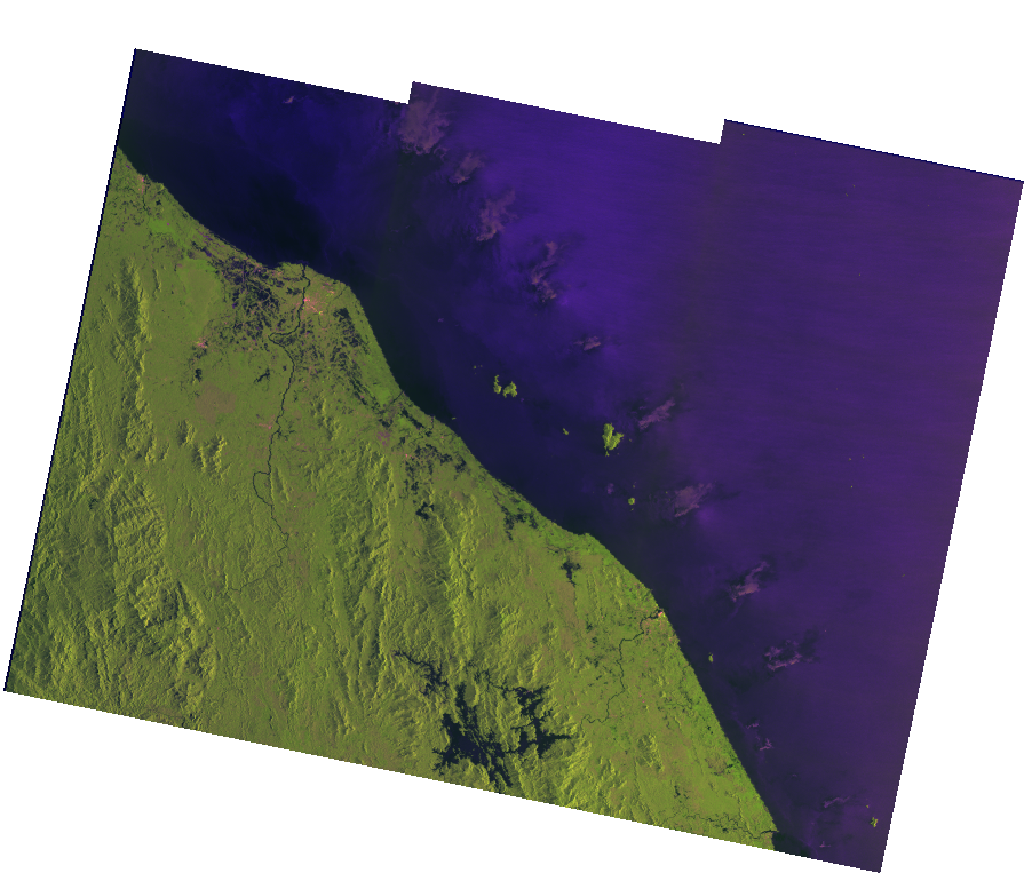
In this case study, we’ll look at the flood water extent over the Narathiwat Province in Thailand 🇹🇭 and the Northern Kelantan State in Malaysia 🇲🇾 on 04 Jan 2017 that were digitized by 🇺🇳 UNITAR-UNOSAT’s rapid mapping service over Synthetic Aperture Radar (SAR) 🛰️ images. Specifically, we’ll be using the 🇪🇺 Sentinel-1 Ground Range Detected (GRD) product’s VV polarization channel.
🔗 Links:
To start, let’s get the 🛰️ satellite scene we’ll be using for this tutorial.
item_url = "https://planetarycomputer.microsoft.com/api/stac/v1/collections/sentinel-1-grd/items/S1A_IW_GRDH_1SDV_20170104T225443_20170104T225512_014688_017E5D"

# Load the individual item metadata and sign the assets
item = pystac.Item.from_file(item_url)
signed_item = planetary_computer.sign(item)
signed_item
- type "Feature"
- stac_version "1.0.0"
- id "S1A_IW_GRDH_1SDV_20170104T225443_20170104T225512_014688_017E5D"
properties
- datetime "2017-01-04T22:54:58.307768Z"
- platform "SENTINEL-1A"
s1:shape[] 2 items
- 0 25293
- 1 19536
- end_datetime "2017-01-04 22:55:12.816643+00:00"
- constellation "Sentinel-1"
- s1:resolution "high"
- s1:datatake_id "97885"
- start_datetime "2017-01-04 22:54:43.798893+00:00"
- s1:orbit_source "RESORB"
- s1:slice_number "1"
- s1:total_slices "7"
- sar:looks_range 5
- sat:orbit_state "descending"
- sar:product_type "GRD"
- sar:looks_azimuth 1
sar:polarizations[] 2 items
- 0 "VV"
- 1 "VH"
- sar:frequency_band "C"
- sat:absolute_orbit 14688
- sat:relative_orbit 91
- s1:processing_level "1"
- sar:instrument_mode "IW"
- sar:center_frequency 5.405
- sar:resolution_range 20
- s1:product_timeliness "Fast-24h"
- sar:resolution_azimuth 22
- sar:pixel_spacing_range 10
- sar:observation_direction "right"
- sar:pixel_spacing_azimuth 10
- sar:looks_equivalent_number 4.4
- s1:instrument_configuration_ID "5"
- sat:platform_international_designator "2014-016A"
geometry
- type "Polygon"
coordinates[] 1 items
0[] 14 items
0[] 2 items
- 0 104.0336434
- 1 6.3096294
1[] 2 items
- 0 103.475118
- 1 6.4251243
2[] 2 items
- 0 102.9150114
- 1 6.5402769
3[] 2 items
- 0 102.354648
- 1 6.6548009
4[] 2 items
- 0 101.8103367
- 1 6.7653797
5[] 2 items
- 0 101.6521135
- 1 5.9820791
6[] 2 items
- 0 101.5785254
- 1 5.6200584
7[] 2 items
- 0 101.5411206
- 1 5.4391662
8[] 2 items
- 0 101.4773595
- 1 5.1372729
9[] 2 items
- 0 102.5782923
- 1 4.9096554
10[] 2 items
- 0 103.6933788
- 1 4.6770784
11[] 2 items
- 0 103.758411
- 1 4.9797866
12[] 2 items
- 0 103.796571
- 1 5.1611755
13[] 2 items
- 0 104.0336434
- 1 6.3096294
links[] 6 items
0
- rel "self"
- href "https://planetarycomputer.microsoft.com/api/stac/v1/collections/sentinel-1-grd/items/S1A_IW_GRDH_1SDV_20170104T225443_20170104T225512_014688_017E5D"
- type "application/json"
1
- rel "collection"
- href "https://planetarycomputer.microsoft.com/api/stac/v1/collections/sentinel-1-grd"
- type "application/json"
2
- rel "parent"
- href "https://planetarycomputer.microsoft.com/api/stac/v1/collections/sentinel-1-grd"
- type "application/json"
3
- rel "root"
- href "https://planetarycomputer.microsoft.com/api/stac/v1/"
- type "application/json"
4
- rel "license"
- href "https://sentinel.esa.int/documents/247904/690755/Sentinel_Data_Legal_Notice"
5
- rel "preview"
- href "https://planetarycomputer.microsoft.com/api/data/v1/item/map?collection=sentinel-1-grd&item=S1A_IW_GRDH_1SDV_20170104T225443_20170104T225512_014688_017E5D"
- type "text/html"
- title "Map of item"
assets
vh
- href "https://sentinel1euwest.blob.core.windows.net/s1-grd/GRD/2017/1/4/IW/DV/S1A_IW_GRDH_1SDV_20170104T225443_20170104T225512_014688_017E5D_6D3B/measurement/iw-vh.tiff?st=2024-04-11T07%3A12%3A23Z&se=2024-04-13T07%3A12%3A23Z&sp=rl&sv=2021-06-08&sr=c&skoid=c85c15d6-d1ae-42d4-af60-e2ca0f81359b&sktid=72f988bf-86f1-41af-91ab-2d7cd011db47&skt=2024-04-11T21%3A14%3A02Z&ske=2024-04-18T21%3A14%3A02Z&sks=b&skv=2021-06-08&sig=8xqtHe9ZqN1XSgzTvpm8yWLqMJ3TVQz6Xzk7uFJ4zhI%3D"
- type "image/tiff; application=geotiff; profile=cloud-optimized"
- title "VH: vertical transmit, horizontal receive"
- description "Amplitude of signal transmitted with vertical polarization and received with horizontal polarization with radiometric terrain correction applied."
roles[] 1 items
- 0 "data"
vv
- href "https://sentinel1euwest.blob.core.windows.net/s1-grd/GRD/2017/1/4/IW/DV/S1A_IW_GRDH_1SDV_20170104T225443_20170104T225512_014688_017E5D_6D3B/measurement/iw-vv.tiff?st=2024-04-11T07%3A12%3A23Z&se=2024-04-13T07%3A12%3A23Z&sp=rl&sv=2021-06-08&sr=c&skoid=c85c15d6-d1ae-42d4-af60-e2ca0f81359b&sktid=72f988bf-86f1-41af-91ab-2d7cd011db47&skt=2024-04-11T21%3A14%3A02Z&ske=2024-04-18T21%3A14%3A02Z&sks=b&skv=2021-06-08&sig=8xqtHe9ZqN1XSgzTvpm8yWLqMJ3TVQz6Xzk7uFJ4zhI%3D"
- type "image/tiff; application=geotiff; profile=cloud-optimized"
- title "VV: vertical transmit, vertical receive"
- description "Amplitude of signal transmitted with vertical polarization and received with vertical polarization with radiometric terrain correction applied."
roles[] 1 items
- 0 "data"
thumbnail
- href "https://sentinel1euwest.blob.core.windows.net/s1-grd/GRD/2017/1/4/IW/DV/S1A_IW_GRDH_1SDV_20170104T225443_20170104T225512_014688_017E5D_6D3B/preview/quick-look.png?st=2024-04-11T07%3A12%3A23Z&se=2024-04-13T07%3A12%3A23Z&sp=rl&sv=2021-06-08&sr=c&skoid=c85c15d6-d1ae-42d4-af60-e2ca0f81359b&sktid=72f988bf-86f1-41af-91ab-2d7cd011db47&skt=2024-04-11T21%3A14%3A02Z&ske=2024-04-18T21%3A14%3A02Z&sks=b&skv=2021-06-08&sig=8xqtHe9ZqN1XSgzTvpm8yWLqMJ3TVQz6Xzk7uFJ4zhI%3D"
- type "image/png"
- title "Preview Image"
- description "An averaged, decimated preview image in PNG format. Single polarisation products are represented with a grey scale image. Dual polarisation products are represented by a single composite colour image in RGB with the red channel (R) representing the co-polarisation VV or HH), the green channel (G) represents the cross-polarisation (VH or HV) and the blue channel (B) represents the ratio of the cross an co-polarisations."
roles[] 1 items
- 0 "thumbnail"
safe-manifest
- href "https://sentinel1euwest.blob.core.windows.net/s1-grd/GRD/2017/1/4/IW/DV/S1A_IW_GRDH_1SDV_20170104T225443_20170104T225512_014688_017E5D_6D3B/manifest.safe?st=2024-04-11T07%3A12%3A23Z&se=2024-04-13T07%3A12%3A23Z&sp=rl&sv=2021-06-08&sr=c&skoid=c85c15d6-d1ae-42d4-af60-e2ca0f81359b&sktid=72f988bf-86f1-41af-91ab-2d7cd011db47&skt=2024-04-11T21%3A14%3A02Z&ske=2024-04-18T21%3A14%3A02Z&sks=b&skv=2021-06-08&sig=8xqtHe9ZqN1XSgzTvpm8yWLqMJ3TVQz6Xzk7uFJ4zhI%3D"
- type "application/xml"
- title "Manifest File"
- description "General product metadata in XML format. Contains a high-level textual description of the product and references to all of product's components, the product metadata, including the product identification and the resource references, and references to the physical location of each component file contained in the product."
roles[] 1 items
- 0 "metadata"
schema-noise-vh
- href "https://sentinel1euwest.blob.core.windows.net/s1-grd/GRD/2017/1/4/IW/DV/S1A_IW_GRDH_1SDV_20170104T225443_20170104T225512_014688_017E5D_6D3B/annotation/calibration/noise-iw-vh.xml?st=2024-04-11T07%3A12%3A23Z&se=2024-04-13T07%3A12%3A23Z&sp=rl&sv=2021-06-08&sr=c&skoid=c85c15d6-d1ae-42d4-af60-e2ca0f81359b&sktid=72f988bf-86f1-41af-91ab-2d7cd011db47&skt=2024-04-11T21%3A14%3A02Z&ske=2024-04-18T21%3A14%3A02Z&sks=b&skv=2021-06-08&sig=8xqtHe9ZqN1XSgzTvpm8yWLqMJ3TVQz6Xzk7uFJ4zhI%3D"
- type "application/xml"
- title "Noise Schema"
- description "Estimated thermal noise look-up tables"
roles[] 1 items
- 0 "metadata"
schema-noise-vv
- href "https://sentinel1euwest.blob.core.windows.net/s1-grd/GRD/2017/1/4/IW/DV/S1A_IW_GRDH_1SDV_20170104T225443_20170104T225512_014688_017E5D_6D3B/annotation/calibration/noise-iw-vv.xml?st=2024-04-11T07%3A12%3A23Z&se=2024-04-13T07%3A12%3A23Z&sp=rl&sv=2021-06-08&sr=c&skoid=c85c15d6-d1ae-42d4-af60-e2ca0f81359b&sktid=72f988bf-86f1-41af-91ab-2d7cd011db47&skt=2024-04-11T21%3A14%3A02Z&ske=2024-04-18T21%3A14%3A02Z&sks=b&skv=2021-06-08&sig=8xqtHe9ZqN1XSgzTvpm8yWLqMJ3TVQz6Xzk7uFJ4zhI%3D"
- type "application/xml"
- title "Noise Schema"
- description "Estimated thermal noise look-up tables"
roles[] 1 items
- 0 "metadata"
schema-product-vh
- href "https://sentinel1euwest.blob.core.windows.net/s1-grd/GRD/2017/1/4/IW/DV/S1A_IW_GRDH_1SDV_20170104T225443_20170104T225512_014688_017E5D_6D3B/annotation/iw-vh.xml?st=2024-04-11T07%3A12%3A23Z&se=2024-04-13T07%3A12%3A23Z&sp=rl&sv=2021-06-08&sr=c&skoid=c85c15d6-d1ae-42d4-af60-e2ca0f81359b&sktid=72f988bf-86f1-41af-91ab-2d7cd011db47&skt=2024-04-11T21%3A14%3A02Z&ske=2024-04-18T21%3A14%3A02Z&sks=b&skv=2021-06-08&sig=8xqtHe9ZqN1XSgzTvpm8yWLqMJ3TVQz6Xzk7uFJ4zhI%3D"
- type "application/xml"
- title "Product Schema"
- description "Describes the main characteristics corresponding to the band: state of the platform during acquisition, image properties, Doppler information, geographic location, etc."
roles[] 1 items
- 0 "metadata"
schema-product-vv
- href "https://sentinel1euwest.blob.core.windows.net/s1-grd/GRD/2017/1/4/IW/DV/S1A_IW_GRDH_1SDV_20170104T225443_20170104T225512_014688_017E5D_6D3B/annotation/iw-vv.xml?st=2024-04-11T07%3A12%3A23Z&se=2024-04-13T07%3A12%3A23Z&sp=rl&sv=2021-06-08&sr=c&skoid=c85c15d6-d1ae-42d4-af60-e2ca0f81359b&sktid=72f988bf-86f1-41af-91ab-2d7cd011db47&skt=2024-04-11T21%3A14%3A02Z&ske=2024-04-18T21%3A14%3A02Z&sks=b&skv=2021-06-08&sig=8xqtHe9ZqN1XSgzTvpm8yWLqMJ3TVQz6Xzk7uFJ4zhI%3D"
- type "application/xml"
- title "Product Schema"
- description "Describes the main characteristics corresponding to the band: state of the platform during acquisition, image properties, Doppler information, geographic location, etc."
roles[] 1 items
- 0 "metadata"
schema-calibration-vh
- href "https://sentinel1euwest.blob.core.windows.net/s1-grd/GRD/2017/1/4/IW/DV/S1A_IW_GRDH_1SDV_20170104T225443_20170104T225512_014688_017E5D_6D3B/annotation/calibration/calibration-iw-vh.xml?st=2024-04-11T07%3A12%3A23Z&se=2024-04-13T07%3A12%3A23Z&sp=rl&sv=2021-06-08&sr=c&skoid=c85c15d6-d1ae-42d4-af60-e2ca0f81359b&sktid=72f988bf-86f1-41af-91ab-2d7cd011db47&skt=2024-04-11T21%3A14%3A02Z&ske=2024-04-18T21%3A14%3A02Z&sks=b&skv=2021-06-08&sig=8xqtHe9ZqN1XSgzTvpm8yWLqMJ3TVQz6Xzk7uFJ4zhI%3D"
- type "application/xml"
- title "Calibration Schema"
- description "Calibration metadata including calibration information and the beta nought, sigma nought, gamma and digital number look-up tables that can be used for absolute product calibration."
roles[] 1 items
- 0 "metadata"
schema-calibration-vv
- href "https://sentinel1euwest.blob.core.windows.net/s1-grd/GRD/2017/1/4/IW/DV/S1A_IW_GRDH_1SDV_20170104T225443_20170104T225512_014688_017E5D_6D3B/annotation/calibration/calibration-iw-vv.xml?st=2024-04-11T07%3A12%3A23Z&se=2024-04-13T07%3A12%3A23Z&sp=rl&sv=2021-06-08&sr=c&skoid=c85c15d6-d1ae-42d4-af60-e2ca0f81359b&sktid=72f988bf-86f1-41af-91ab-2d7cd011db47&skt=2024-04-11T21%3A14%3A02Z&ske=2024-04-18T21%3A14%3A02Z&sks=b&skv=2021-06-08&sig=8xqtHe9ZqN1XSgzTvpm8yWLqMJ3TVQz6Xzk7uFJ4zhI%3D"
- type "application/xml"
- title "Calibration Schema"
- description "Calibration metadata including calibration information and the beta nought, sigma nought, gamma and digital number look-up tables that can be used for absolute product calibration."
roles[] 1 items
- 0 "metadata"
tilejson
- href "https://planetarycomputer.microsoft.com/api/data/v1/item/tilejson.json?collection=sentinel-1-grd&item=S1A_IW_GRDH_1SDV_20170104T225443_20170104T225512_014688_017E5D&assets=vv&assets=vh&expression=vv%3Bvh%3Bvv%2Fvh&rescale=0%2C600&rescale=0%2C270&rescale=0%2C9&asset_as_band=True&tile_format=png&format=png"
- type "application/json"
- title "TileJSON with default rendering"
roles[] 1 items
- 0 "tiles"
rendered_preview
- href "https://planetarycomputer.microsoft.com/api/data/v1/item/preview.png?collection=sentinel-1-grd&item=S1A_IW_GRDH_1SDV_20170104T225443_20170104T225512_014688_017E5D&assets=vv&assets=vh&expression=vv%3Bvh%3Bvv%2Fvh&rescale=0%2C600&rescale=0%2C270&rescale=0%2C9&asset_as_band=True&tile_format=png&format=png"
- type "image/png"
- title "Rendered preview"
- rel "preview"
roles[] 1 items
- 0 "overview"
bbox[] 4 items
- 0 101.47735954
- 1 4.67707843
- 2 104.03364342
- 3 6.76537966
stac_extensions[] 3 items
- 0 "https://stac-extensions.github.io/sar/v1.0.0/schema.json"
- 1 "https://stac-extensions.github.io/sat/v1.0.0/schema.json"
- 2 "https://stac-extensions.github.io/eo/v1.1.0/schema.json"
- collection "sentinel-1-grd"
This is how the Sentinel-1 🩻 image looks like over Southern Thailand / Northern Peninsular Malaysia on 04 Jan 2017.
Load and reproject image data 🔄#
To keep things simple, we’ll load just the VV channel into a DataPipe via
zen3geo.datapipes.RioXarrayReader (functional name:
read_from_rioxarray) 😀.
url = signed_item.assets["vv"].href
dp = torchdata.datapipes.iter.IterableWrapper(iterable=[url])
# Reading lower resolution grid using overview_level=3
dp_rioxarray = dp.read_from_rioxarray(overview_level=3)
dp_rioxarray
RioXarrayReaderIterDataPipe
The Sentinel-1 image from Planetary Computer comes in longitude/latitude 🌐 geographic coordinates by default (OGC:CRS84). To make the pixels more equal 🔲 area, we can project it to a 🌏 local projected coordinate system instead.
def reproject_to_local_utm(dataarray: xr.DataArray, resolution: float=80.0) -> xr.DataArray:
    """
    Reproject an xarray.DataArray grid from OGC:CRS84 to a local UTM coordinate
    reference system.
    """
    # Estimate UTM coordinate reference from a single pixel
    pixel = dataarray.isel(y=slice(0, 1), x=slice(0,1))
    new_crs = dataarray.rio.reproject(dst_crs="OGC:CRS84").rio.estimate_utm_crs()

    return dataarray.rio.reproject(dst_crs=new_crs, resolution=resolution)
dp_reprojected = dp_rioxarray.map(fn=reproject_to_local_utm)
Note
Universal Transverse Mercator (UTM) isn’t actually an equal-area projection system. However, Sentinel-1 🛰️ satellite scenes from Copernicus are usually distributed in a UTM coordinate reference system, and UTM is typically a close enough 🤏 approximation to the local geographic area, or at least it won’t matter much when we’re looking at spatial resolutions over several 10s of metres 🙂.
Hint
For those wondering what OGC:CRS84 is, it is the longitude/latitude version
of EPSG:4326 🌐 (latitude/longitude). I.e., it’s a
matter of axis order, with OGC:CRS84 being x/y and EPSG:4326 being y/x.
🔖 References:
Transform and visualize raster data 🔎#
Let’s visualize 👀 the Sentinel-1 image, but before that, we’ll transform 🔄 the VV data from linear to decibel scale.
def linear_to_decibel(dataarray: xr.DataArray) -> xr.DataArray:
    """
    Transforming the input xarray.DataArray's VV or VH values from linear to
    decibel scale using the formula ``10 * log_10(x)``.
    """
    # Mask out areas with 0 so that np.log10 is not undefined
    da_linear = dataarray.where(cond=dataarray != 0)
    da_decibel = 10 * np.log10(da_linear)
    return da_decibel
dp_decibel = dp_reprojected.map(fn=linear_to_decibel)
dp_decibel
MapperIterDataPipe
As an aside, we’ll be using the Sentinel-1 image datapipe twice later, once as
a template to create a blank canvas 🎞️, and another time by itself 🪞. This
requires forking 🍴 the DataPipe into two branches, which can be achieved using
torchdata.datapipes.iter.Forker (functional name: fork).
dp_decibel_canvas, dp_decibel_image = dp_decibel.fork(num_instances=2)
dp_decibel_canvas, dp_decibel_image
(_ChildDataPipe, _ChildDataPipe)
Now to visualize the transformed Sentinel-1 image 🖼️. Let’s zoom in 🔭 to one of the analysis extent areas we’ll be working on later.
it = iter(dp_decibel_image)
dataarray = next(it)

da_clip = dataarray.rio.clip_box(minx=125718, miny=523574, maxx=326665, maxy=722189)
da_clip.isel(band=0).plot.imshow(figsize=(11.5, 9), cmap="Blues_r", vmin=18, vmax=26)
<matplotlib.image.AxesImage at 0x7f7e379a2810>
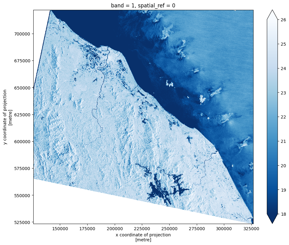
Notice how the darker blue areas 🔵 tend to correlate more with water features like the meandering rivers and the 🐚 sea on the NorthEast. This is because the SAR 🛰️ signal which is side looking reflects off flat water bodies like a mirror 🪞, with little energy getting reflected 🙅 back directly to the sensor (hence why it looks darker ⚫).
Load and visualize cloud-hosted vector files 💠#
Let’s now load some vector data from the web 🕸️. These are polygons of the segmented 🌊 water extent digitized by UNOSAT’s AI Based Rapid Mapping Service. We’ll be converting these vector polygons to 🌈 raster masks later.
🔗 Links:
# https://gdal.org/user/virtual_file_systems.html#vsizip-zip-archives
shape_url = "/vsizip/vsicurl/https://web.archive.org/web/20240411214446/https://unosat.org/static/unosat_filesystem/2460/FL20170106THA_SHP.zip/ST20170104_SatelliteDetectedWaterAndSaturatedSoil.shp"
This is a shapefile containing 🔷 polygons of the mapped water extent. Let’s
put it into a DataPipe called zen3geo.datapipes.PyogrioReader
(functional name: read_from_pyogrio).
dp_shapes = torchdata.datapipes.iter.IterableWrapper(iterable=[shape_url])
dp_pyogrio = dp_shapes.read_from_pyogrio()
dp_pyogrio
PyogrioReaderIterDataPipe
This will take care of loading the shapefile into a
geopandas.GeoDataFrame object. Let’s take a look at the data table
📊 to see what attributes are inside.
it = iter(dp_pyogrio)
geodataframe = next(it)
geodataframe.dropna(axis="columns")
/home/docs/checkouts/readthedocs.org/user_builds/zen3geo/envs/latest/lib/python3.11/site-packages/pyogrio/geopandas.py:49: FutureWarning: errors='ignore' is deprecated and will raise in a future version. Use to_datetime without passing `errors` and catch exceptions explicitly instead
  res = pd.to_datetime(ser, **datetime_kwargs)
| Water_Clas | Sensor_ID | Sensor_Dat | Confidence | Field_Vali | Water_Stat | Area_m2 | Area_ha | StaffID | EventCode | |
|---|---|---|---|---|---|---|---|---|---|---|
| 0 | Satellite Detected Water | Sentinel-1 | 2017-01-04 | Medium | Not yet field validated | New Water / Water Increase | 1701.928663 | 0.170193 | AM | FL20170106THA |
| 1 | Satellite Detected Water | Sentinel-1 | 2017-01-04 | Medium | Not yet field validated | New Water / Water Increase | 782.018715 | 0.078202 | AM | FL20170106THA |
| 2 | Satellite Detected Water | Sentinel-1 | 2017-01-04 | Medium | Not yet field validated | New Water / Water Increase | 918.165480 | 0.091817 | AM | FL20170106THA |
| 3 | Satellite Detected Water | Sentinel-1 | 2017-01-04 | Medium | Not yet field validated | New Water / Water Increase | 809.427244 | 0.080943 | AM | FL20170106THA |
| 4 | Satellite Detected Water | Sentinel-1 | 2017-01-04 | Medium | Not yet field validated | New Water / Water Increase | 1299.320215 | 0.129932 | AM | FL20170106THA |
| ... | ... | ... | ... | ... | ... | ... | ... | ... | ... | ... |
| 25487 | Satellite Detected Water | Sentinel-1 | 2017-01-04 | Medium | Not yet field validated | New Water / Water Increase | 12536.344160 | 1.253634 | AM | FL20170106THA |
| 25488 | Satellite Detected Water | Sentinel-1 | 2017-01-04 | Medium | Not yet field validated | New Water / Water Increase | 10029.167383 | 1.002917 | AM | FL20170106THA |
| 25489 | Satellite Detected Water | Sentinel-1 | 2017-01-04 | Medium | Not yet field validated | New Water / Water Increase | 212535.649717 | 21.253565 | AM | FL20170106THA |
| 25490 | Satellite Detected Water | Sentinel-1 | 2017-01-04 | Medium | Not yet field validated | New Water / Water Increase | 130468.805286 | 13.046881 | AM | FL20170106THA |
| 25491 | Satellite Detected Water | Sentinel-1 | 2017-01-04 | Medium | Not yet field validated | New Water / Water Increase | 74465.781664 | 7.446578 | AM | FL20170106THA |
25492 rows × 10 columns
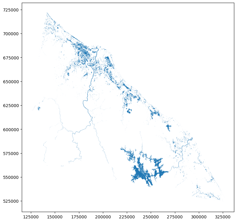
Cool, and we can also visualize the polygons 🔷 on a 2D map. To align the
coordinates with the 🛰️ Sentinel-1 image above, we’ll first use
geopandas.GeoDataFrame.to_crs() to reproject the vector from 🌐
EPSG:9707 (WGS 84 + EGM96 height, latitude/longitude) to 🌏 EPSG:32648 (UTM
Zone 48N).
print(f"Original bounds in EPSG:9707:\n{geodataframe.bounds}")
gdf = geodataframe.to_crs(crs="EPSG:32648")
print(f"New bounds in EPSG:32648:\n{gdf.bounds}")
Original bounds in EPSG:9707:
             minx      miny        maxx      maxy
0      103.402642  4.780603  103.404319  4.781299
1      103.404618  4.781411  103.405402  4.781838
2      103.424314  4.811825  103.424717  4.812201
3      103.361522  4.921706  103.361921  4.922521
4      103.335201  4.968863  103.336148  4.970452
...           ...       ...         ...       ...
25487  103.300346  5.022766  103.303215  5.023847
25488  103.337896  4.962220  103.338974  4.963702
25489  103.374996  4.876161  103.387663  4.896643
25490  101.952245  6.330713  101.958892  6.337442
25491  101.906520  6.377672  101.913865  6.386013

[25492 rows x 4 columns]
New bounds in EPSG:32648:
                minx           miny           maxx           maxy
0      322845.475538  528618.384523  323031.725338  528695.041456
1      323064.876388  528707.234812  323152.040798  528754.319128
2      325257.557428  532065.352157  325302.408278  532106.948358
3      318321.778598  544232.596674  318365.870200  544322.812408
4      315415.721730  549454.566256  315520.394144  549630.461524
...              ...            ...            ...            ...
25487  311565.178818  555425.372112  311883.321090  555544.434637
25488  315712.560200  548719.127186  315832.015625  548883.087763
25489  319809.244128  539189.350228  321208.958886  541457.480945
25490  162763.145300  700749.683788  163497.165363  701496.603781
25491  157731.551740  705975.835176  158539.411335  706904.040326

[25492 rows x 4 columns]
Plot it with geopandas.GeoDataFrame.plot(). This vector map 🗺️ should
correspond to the zoomed in Sentinel-1 image plotted earlier above.
gdf.plot(figsize=(11.5, 9))
<Axes: >
Tip
Make sure to understand your raster and vector datasets well first! Open the files up in your favourite 🌐 Geographic Information System (GIS) tool, see how they actually look like spatially. Then you’ll have a better idea to decide on how to create your data pipeline. The zen3geo way puts you as the Master 🧙 in control.
1️⃣ Create a canvas to paint on 🎨#
In this section, we’ll work on converting the flood water 🌊 polygons above from a 🚩 vector to a 🌈 raster format, i.e. rasterization. This will be done in two steps 📶:
Defining a blank canvas 🎞️
Paint the polygons onto this blank canvas 🧑🎨
For this, we’ll be using tools from zen3geo.datapipes.datashader().
Let’s see how this can be done.
Blank canvas from template raster 🖼️#
A canvas represents a 2D area with a height and a width 📏. For us, we’ll be
using a datashader.Canvas, which also defines the range of y-values
(ymin to ymax) and x-values (xmin to xmax), essentially coordinates for
every unit 🇾 height and 🇽 width.
Since we already have a Sentinel-1 🛰️ raster grid with defined height/width
and y/x coordinates, let’s use it as a 📄 template to define our canvas. This
is done via zen3geo.datapipes.XarrayCanvas (functional name:
canvas_from_xarray).
dp_canvas = dp_decibel_canvas.canvas_from_xarray()
dp_canvas
XarrayCanvasIterDataPipe
Cool, and here’s a quick inspection 👀 of the canvas dimensions and metadata.
it = iter(dp_canvas)
canvas = next(it)
print(f"Canvas height: {canvas.plot_height}, width: {canvas.plot_width}")
print(f"Y-range: {canvas.y_range}")
print(f"X-range: {canvas.x_range}")
print(f"Coordinate reference system: {canvas.crs}")
Canvas height: 3073, width: 3606
Y-range: (516991.17434596806, 762831.1743459681)
X-range: (107650.27505862404, 396130.27505862404)
Coordinate reference system: EPSG:32648
This information should match the template Sentinel-1 dataarray 🏁.
print(f"Dimensions: {dict(dataarray.sizes)}")
print(f"Affine transform: {dataarray.rio.transform()}")
print(f"Bounding box: {dataarray.rio.bounds()}")
print(f"Coordinate reference system: {dataarray.rio.crs}")
Dimensions: {'band': 1, 'y': 3073, 'x': 3606}
Affine transform: | 80.00, 0.00, 107650.28|
| 0.00,-80.00, 762831.17|
| 0.00, 0.00, 1.00|
Bounding box: (107650.27505862404, 516991.17434596806, 396130.27505862404, 762831.1743459681)
Coordinate reference system: EPSG:32648
Rasterize vector polygons onto canvas 🖌️#
Now’s the time to paint or rasterize the
vector geopandas.GeoDataFrame polygons 🔷 onto the blank
datashader.Canvas! This would enable us to have a direct pixel-wise
X -> Y mapping ↔️ between the Sentinel-1 image (X) and target flood label (Y).
The vector polygons can be rasterized or painted 🖌️ onto the template canvas
using zen3geo.datapipes.DatashaderRasterizer (functional name:
rasterize_with_datashader).
dp_datashader = dp_canvas.rasterize_with_datashader(vector_datapipe=dp_pyogrio)
dp_datashader
DatashaderRasterizerIterDataPipe
This will turn the vector geopandas.GeoDataFrame into a
raster xarray.DataArray grid, with the spatial coordinates and
bounds matching exactly with the template Sentinel-1 image 😎.
Note
Since we have just one Sentinel-1 🛰️ image and one raster 💧 flood
mask, we have an easy 1:1 mapping. There are two other scenarios supported by
zen3geo.datapipes.DatashaderRasterizer:
N:1 - Many
datashader.Canvasobjects to one vectorgeopandas.GeoDataFrame. The single vector geodataframe will be broadcasted to match the length of the canvas list. This is useful for situations when you have a 🌐 ‘global’ vector database that you want to pair with multiple 🛰️ satellite images.N:N - Many
datashader.Canvasobjects to many vectorgeopandas.GeoDataFrameobjects. In this case, the list of grids must ❗ have the same length as the list of vector geodataframes. E.g. if you have 5 grids, there must also be 5 vector files. This is so that a 1:1 pairing can be done, useful when each raster tile 🖽 has its own associated vector annotation.
See also
For more details on how rasterization of polygons work behind the scenes 🎦, check out Datashader’s documentation on:
The datashader pipeline (especially the section on Aggregation).
2️⃣ Combine and conquer ⚔️#
So far, we’ve got two datapipes that should be 🧑🤝🧑 paired up in an X -> Y manner:
The pre-processed Sentinel-1 🌈 raster image in
dp_decibel_imageThe rasterized 💧 flood segmentation masks in
dp_datashader
One way to get these two pieces in a Machine Learning ready chip format is via a stack, slice and split ™️ approach. Think of it like a sandwich 🥪, we first stack the bread 🍞 and lettuce 🥬, and then slice the pieces 🍕 through the layers once. Ok, that was a bad analogy, let’s just stick with tensors 🤪.
Stacking the raster layers 🥞#
Each of our 🌈 raster inputs are xarray.DataArray objects with the
same spatial resolution and extent 🪟, so these can be stacked into an
xarray.Dataset with multiple data variables. First, we’ll zip 🤐
the two datapipes together using torchdata.datapipes.iter.Zipper
(functional name: zip)
dp_zip = dp_decibel_image.zip(dp_datashader)
dp_zip
ZipperIterDataPipe
This will result in a DataPipe where each item is a tuple of (X, Y) pairs 🧑🤝🧑.
Just to illustrate what we’ve done so far, we can use
torchdata.datapipes.utils.to_graph to visualize the data pipeline
⛓️.
torchdata.datapipes.utils.to_graph(dp=dp_zip)

Next, let’s combine 🖇️ the two (X, Y) xarray.DataArray objects in
the tuple into an xarray.Dataset using
torchdata.datapipes.iter.Collator (functional name: collate).
We’ll also ✂️ clip the dataset to a bounding box area where the target water
mask has no 0 or NaN values.
def xr_collate_fn(image_and_mask: tuple) -> xr.Dataset:
    """
    Combine a pair of xarray.DataArray (image, mask) inputs into an
    xarray.Dataset with two data variables named 'image' and 'mask'.
    """
    # Turn 2 xr.DataArray objects into 1 xr.Dataset with multiple data vars
    image, mask = image_and_mask
    dataset: xr.Dataset = xr.merge(
        objects=[image.isel(band=0).rename("image"), mask.rename("mask")],
        join="override",
    )

    # Clip dataset to bounding box extent of where labels are
    mask_extent: tuple = mask.where(cond=mask == 1, drop=True).rio.bounds()
    clipped_dataset: xr.Dataset = dataset.rio.clip_box(*mask_extent)

    return clipped_dataset
dp_dataset = dp_zip.collate(collate_fn=xr_collate_fn)
dp_dataset
CollatorIterDataPipe
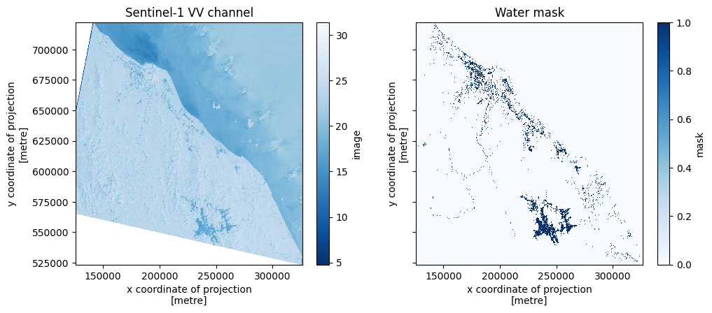
Double check to see that resulting xarray.Dataset’s image and mask
looks ok 🙆♂️.
it = iter(dp_dataset)
dataset = next(it)

# Create subplot with VV image on the left and Water mask on the right
fig, axs = plt.subplots(ncols=2, figsize=(11.5, 4.5), sharey=True)
dataset.image.plot.imshow(ax=axs[0], cmap="Blues_r")
axs[0].set_title("Sentinel-1 VV channel")
dataset.mask.plot.imshow(ax=axs[1], cmap="Blues")
axs[1].set_title("Water mask")
plt.show()
/home/docs/checkouts/readthedocs.org/user_builds/zen3geo/envs/latest/lib/python3.11/site-packages/torch/utils/data/datapipes/iter/combining.py:337: UserWarning: Some child DataPipes are not exhausted when __iter__ is called. We are resetting the buffer and each child DataPipe will read from the start again.
  warnings.warn("Some child DataPipes are not exhausted when __iter__ is called. We are resetting "
/home/docs/checkouts/readthedocs.org/user_builds/zen3geo/envs/latest/lib/python3.11/site-packages/pyogrio/geopandas.py:49: FutureWarning: errors='ignore' is deprecated and will raise in a future version. Use to_datetime without passing `errors` and catch exceptions explicitly instead
  res = pd.to_datetime(ser, **datetime_kwargs)
Slice into chips and turn into tensors 🗡️#
To cut 🔪 the xarray.Dataset into 512x512 sized chips, we’ll use
zen3geo.datapipes.XbatcherSlicer (functional name:
slice_with_xbatcher). Refer to Chipping and batching data if you need a 🧑🎓 refresher.
dp_xbatcher = dp_dataset.slice_with_xbatcher(input_dims={"y": 512, "x": 512})
dp_xbatcher
XbatcherSlicerIterDataPipe
Next step is to convert the 512x512 chips into a torch.Tensor via
torchdata.datapipes.iter.Mapper (functional name: map). The 🛰️
Sentinel-1 image and 💧 water mask will be split out at this point too.
def dataset_to_tensors(chip: xr.Dataset) -> (torch.Tensor, torch.Tensor):
    """
    Converts an xarray.Dataset into to two torch.Tensor objects, the first one
    being the satellite image, and the second one being the target mask.
    """
    image: torch.Tensor = torch.as_tensor(chip.image.data)
    mask: torch.Tensor = torch.as_tensor(chip.mask.data.astype("uint8"))

    return image, mask
dp_map = dp_xbatcher.map(fn=dataset_to_tensors)
dp_map
MapperIterDataPipe
At this point, we could do some batching and collating, but we’ll point you again to Chipping and batching data to figure it out 😝. Let’s take a look at a graph of the complete data pipeline.
torchdata.datapipes.utils.to_graph(dp=dp_map)

Sweet, time for the final step ⏩.
Into a DataLoader 🏋️#
Pass the DataPipe into torch.utils.data.DataLoader 🤾!
dataloader = torch.utils.data.DataLoader(dataset=dp_map)
for i, batch in enumerate(dataloader):
    image, mask = batch
    print(f"Batch {i} - image: {image.shape}, mask: {mask.shape}")
/home/docs/checkouts/readthedocs.org/user_builds/zen3geo/envs/latest/lib/python3.11/site-packages/torch/utils/data/datapipes/iter/combining.py:337: UserWarning: Some child DataPipes are not exhausted when __iter__ is called. We are resetting the buffer and each child DataPipe will read from the start again.
  warnings.warn("Some child DataPipes are not exhausted when __iter__ is called. We are resetting "
/home/docs/checkouts/readthedocs.org/user_builds/zen3geo/envs/latest/lib/python3.11/site-packages/pyogrio/geopandas.py:49: FutureWarning: errors='ignore' is deprecated and will raise in a future version. Use to_datetime without passing `errors` and catch exceptions explicitly instead
  res = pd.to_datetime(ser, **datetime_kwargs)
/home/docs/checkouts/readthedocs.org/user_builds/zen3geo/envs/latest/lib/python3.11/site-packages/pyogrio/geopandas.py:49: FutureWarning: errors='ignore' is deprecated and will raise in a future version. Use to_datetime without passing `errors` and catch exceptions explicitly instead
  res = pd.to_datetime(ser, **datetime_kwargs)
Batch 0 - image: torch.Size([1, 512, 512]), mask: torch.Size([1, 512, 512])
Batch 1 - image: torch.Size([1, 512, 512]), mask: torch.Size([1, 512, 512])
Batch 2 - image: torch.Size([1, 512, 512]), mask: torch.Size([1, 512, 512])
Batch 3 - image: torch.Size([1, 512, 512]), mask: torch.Size([1, 512, 512])
Batch 4 - image: torch.Size([1, 512, 512]), mask: torch.Size([1, 512, 512])
Batch 5 - image: torch.Size([1, 512, 512]), mask: torch.Size([1, 512, 512])
Batch 6 - image: torch.Size([1, 512, 512]), mask: torch.Size([1, 512, 512])
Batch 7 - image: torch.Size([1, 512, 512]), mask: torch.Size([1, 512, 512])
Batch 8 - image: torch.Size([1, 512, 512]), mask: torch.Size([1, 512, 512])
Batch 9 - image: torch.Size([1, 512, 512]), mask: torch.Size([1, 512, 512])
Batch 10 - image: torch.Size([1, 512, 512]), mask: torch.Size([1, 512, 512])
Batch 11 - image: torch.Size([1, 512, 512]), mask: torch.Size([1, 512, 512])
Batch 12 - image: torch.Size([1, 512, 512]), mask: torch.Size([1, 512, 512])
Batch 13 - image: torch.Size([1, 512, 512]), mask: torch.Size([1, 512, 512])
Batch 14 - image: torch.Size([1, 512, 512]), mask: torch.Size([1, 512, 512])
Batch 15 - image: torch.Size([1, 512, 512]), mask: torch.Size([1, 512, 512])
Now go train some flood water detection models 🌊🌊🌊
See also
To learn more about AI-based flood mapping with SAR, check out these resources: