Object detection boxes

You shouldn’t set up limits in boundless openness, but if you set up limitlessness as boundless openness, you’ve trapped yourself

Boxes are quick to draw ✏️, but finicky to train a neural network with. This time, we’ll show you a geospatial object detection 🕵️ problem, where the objects are defined by a bounding box 🔲 with a specific class. By the end of this lesson, you should be able to:

• Read OGR supported vector files and obtain the bounding boxes 🟨 of each geometry

• Convert bounding boxes from geographic coordinates to 🖼️ image coordinates while clipping to the image extent

• Use an affine transform to convert boxes in image coordinates to 🌐 geographic coordinates

🔗 Links:

• https://planetarycomputer.microsoft.com/dataset/ms-buildings#Example-Notebook

• microsoft/GlobalMLBuildingFootprints

• https://mlhub.earth/datasets?tags=object+detection

🎉 Getting started

These are the tools 🛠️ you’ll need.

import contextily
import numpy as np
import geopandas as gpd
import matplotlib.patches
import matplotlib.pyplot as plt
import pandas as pd
import planetary_computer
import pystac_client
import rioxarray
import shapely.affinity
import shapely.geometry
import torch
import torchdata
import torchdata.dataloader2
import xarray as xr
import zen3geo

0️⃣ Find high-resolution imagery and building footprints 🌇

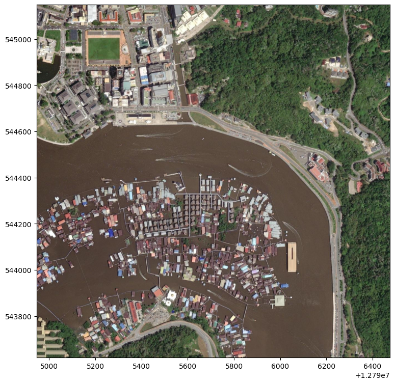
Let’s take a look at buildings over Kampong Ayer, Brunei 🇧🇳! We’ll use contextily.bounds2img() to get some 4-band RGBA 🌈 optical imagery in a numpy.ndarray format.

image, extent = contextily.bounds2img(
    w=114.94,
    s=4.88,
    e=114.95,
    n=4.89,
    ll=True,
    source=contextily.providers.Esri.WorldImagery,
)
print(f"Spatial extent in EPSG:3857: {extent}")
print(f"Image dimensions (height, width, channels): {image.shape}")

Spatial extent in EPSG:3857: (12794947.038712224, 12796475.779277924, 543620.1451641723, 545148.8857298762)
Image dimensions (height, width, channels): (1280, 1280, 4)

This is how Brunei’s 🚣 Venice of the East looks like from above.

fig, ax = plt.subplots(nrows=1, figsize=(9, 9))
plt.imshow(X=image, extent=extent)

<matplotlib.image.AxesImage at 0x7fd055b93a10>

Tip

For more raster basemaps, check out:

• https://xyzservices.readthedocs.io/en/stable/introduction.html#overview-of-built-in-providers

• https://leaflet-extras.github.io/leaflet-providers/preview/

Georeference image using rioxarray 🌐

To enable slicing 🔪 with xbatcher later, we’ll need to turn the numpy.ndarray image 🖼️ into an xarray.DataArray grid with coordinates 🖼️. If you already have a georeferenced grid (e.g. from zen3geo.datapipes.RioXarrayReader), this step can be skipped ⏭️.

# Turn RGBA image from channel-last to channel-first and get 3-band RGB only
_image = image.transpose(2, 0, 1)  # Change image from (H, W, C) to (C, H, W)
rgb_image = _image[0:3, :, :]  # Get just RGB by dropping RGBA's alpha channel
print(f"RGB image shape: {rgb_image.shape}")

RGB image shape: (3, 1280, 1280)

Georeferencing is done by putting the 🚦 RGB image into an xarray.DataArray object with (band, y, x) coordinates, and then setting a coordinate reference system 📐 using rioxarray.rioxarray.XRasterBase.set_crs().

left, right, bottom, top = extent  # xmin, xmax, ymin, ymax
dataarray = xr.DataArray(
    data=rgb_image,
    coords=dict(
        band=[0, 1, 2],  # Red, Green, Blue
        y=np.linspace(start=top, stop=bottom, num=rgb_image.shape[1]),
        x=np.linspace(start=left, stop=right, num=rgb_image.shape[2]),
    ),
    dims=("band", "y", "x"),
)
dataarray = dataarray.rio.write_crs(input_crs="EPSG:3857")
dataarray

<xarray.DataArray (band: 3, y: 1280, x: 1280)>
array([[[111, 105, 105, ...,  40,  67,  81],
        [119, 120, 119, ...,  42,  61,  77],
        [130, 128, 126, ...,  57,  72,  86],
        ...,
        [185, 185, 184, ...,  54,  28,  49],
        [182, 182, 182, ...,  39,  30,  36],
        [181, 181, 181, ...,  30,  58,  70]],

       [[100,  94,  94, ...,  72,  99, 113],
        [107, 109, 108, ...,  72,  93, 109],
        [118, 116, 114, ...,  87, 102, 117],
        ...,
        [178, 178, 177, ...,  75,  49,  70],
        [175, 175, 175, ...,  60,  51,  57],
        [174, 174, 174, ...,  50,  79,  91]],

       [[ 82,  76,  74, ...,  35,  62,  76],
        [ 91,  91,  90, ...,  36,  56,  72],
        [104, 102,  98, ...,  53,  68,  83],
        ...,
        [152, 152, 151, ...,  44,  16,  37],
        [147, 147, 147, ...,  29,  18,  24],
        [146, 146, 146, ...,  22,  48,  58]]], dtype=uint8)
Coordinates:
  * band         (band) int64 0 1 2
  * y            (y) float64 5.451e+05 5.451e+05 ... 5.436e+05 5.436e+05
  * x            (x) float64 1.279e+07 1.279e+07 1.279e+07 ... 1.28e+07 1.28e+07
    spatial_ref  int64 0

xarray.DataArray

• band: 3
• y: 1280
• x: 1280

• 111 105 105 121 141 147 135 119 112 111 ... 41 41 55 65 37 62 22 48 58

  array([[[111, 105, 105, ...,  40,  67,  81],
          [119, 120, 119, ...,  42,  61,  77],
          [130, 128, 126, ...,  57,  72,  86],
          ...,
          [185, 185, 184, ...,  54,  28,  49],
          [182, 182, 182, ...,  39,  30,  36],
          [181, 181, 181, ...,  30,  58,  70]],
  
         [[100,  94,  94, ...,  72,  99, 113],
          [107, 109, 108, ...,  72,  93, 109],
          [118, 116, 114, ...,  87, 102, 117],
          ...,
          [178, 178, 177, ...,  75,  49,  70],
          [175, 175, 175, ...,  60,  51,  57],
          [174, 174, 174, ...,  50,  79,  91]],
  
         [[ 82,  76,  74, ...,  35,  62,  76],
          [ 91,  91,  90, ...,  36,  56,  72],
          [104, 102,  98, ...,  53,  68,  83],
          ...,
          [152, 152, 151, ...,  44,  16,  37],
          [147, 147, 147, ...,  29,  18,  24],
          [146, 146, 146, ...,  22,  48,  58]]], dtype=uint8)

• Coordinates: (4)
  • band
    (band)
    int64
    0 1 2

    array([0, 1, 2])

  • y
    (y)
    float64
    5.451e+05 5.451e+05 ... 5.436e+05

    array([545148.88573 , 545147.690468, 545146.495205, ..., 543622.535689,
           543621.340427, 543620.145164])

  • x
    (x)
    float64
    1.279e+07 1.279e+07 ... 1.28e+07

    array([12794947.038712, 12794948.233975, 12794949.429237, ..., 12796473.388753,
           12796474.584016, 12796475.779278])

  • spatial_ref
    ()
    int64
    0

    crs_wkt :

    PROJCS["WGS 84 / Pseudo-Mercator",GEOGCS["WGS 84",DATUM["WGS_1984",SPHEROID["WGS 84",6378137,298.257223563,AUTHORITY["EPSG","7030"]],AUTHORITY["EPSG","6326"]],PRIMEM["Greenwich",0,AUTHORITY["EPSG","8901"]],UNIT["degree",0.0174532925199433,AUTHORITY["EPSG","9122"]],AUTHORITY["EPSG","4326"]],PROJECTION["Mercator_1SP"],PARAMETER["central_meridian",0],PARAMETER["scale_factor",1],PARAMETER["false_easting",0],PARAMETER["false_northing",0],UNIT["metre",1,AUTHORITY["EPSG","9001"]],AXIS["Easting",EAST],AXIS["Northing",NORTH],EXTENSION["PROJ4","+proj=merc +a=6378137 +b=6378137 +lat_ts=0 +lon_0=0 +x_0=0 +y_0=0 +k=1 +units=m +nadgrids=@null +wktext +no_defs"],AUTHORITY["EPSG","3857"]]

    spatial_ref :

    PROJCS["WGS 84 / Pseudo-Mercator",GEOGCS["WGS 84",DATUM["WGS_1984",SPHEROID["WGS 84",6378137,298.257223563,AUTHORITY["EPSG","7030"]],AUTHORITY["EPSG","6326"]],PRIMEM["Greenwich",0,AUTHORITY["EPSG","8901"]],UNIT["degree",0.0174532925199433,AUTHORITY["EPSG","9122"]],AUTHORITY["EPSG","4326"]],PROJECTION["Mercator_1SP"],PARAMETER["central_meridian",0],PARAMETER["scale_factor",1],PARAMETER["false_easting",0],PARAMETER["false_northing",0],UNIT["metre",1,AUTHORITY["EPSG","9001"]],AXIS["Easting",EAST],AXIS["Northing",NORTH],EXTENSION["PROJ4","+proj=merc +a=6378137 +b=6378137 +lat_ts=0 +lon_0=0 +x_0=0 +y_0=0 +k=1 +units=m +nadgrids=@null +wktext +no_defs"],AUTHORITY["EPSG","3857"]]

    array(0)

• Indexes: (3)
  • band
    PandasIndex

    PandasIndex(Index([0, 1, 2], dtype='int64', name='band'))

  • y
    PandasIndex

    PandasIndex(Index([545148.8857298762, 545147.6904675106, 545146.4952051449,
           545145.2999427792, 545144.1046804135, 545142.9094180479,
           545141.7141556821, 545140.5188933165, 545139.3236309508,
           545138.1283685851,
           ...
           543630.9025254634, 543629.7072630977,  543628.512000732,
           543627.3167383664, 543626.1214760006,  543624.926213635,
           543623.7309512693, 543622.5356889036, 543621.3404265379,
           543620.1451641723],
          dtype='float64', name='y', length=1280))

  • x
    PandasIndex

    PandasIndex(Index([12794947.038712224, 12794948.233974589, 12794949.429236956,
           12794950.624499321, 12794951.819761686, 12794953.015024053,
           12794954.210286418, 12794955.405548783,  12794956.60081115,
           12794957.796073515,
           ...
           12796465.021916633, 12796466.217178999, 12796467.412441365,
            12796468.60770373, 12796469.802966096, 12796470.998228462,
           12796472.193490827, 12796473.388753192,  12796474.58401556,
           12796475.779277924],
          dtype='float64', name='x', length=1280))

• Attributes: (0)

Load cloud-native vector files 💠

Now to pull in some building footprints 🛖. Let’s make a STAC API query to get a GeoParquet file (a cloud-native columnar 🀤 geospatial vector file format) that intersects our study area.

catalog = pystac_client.Client.open(
    url="https://planetarycomputer.microsoft.com/api/stac/v1",
    modifier=planetary_computer.sign_inplace,
)
search = catalog.search(
    collections=["ms-buildings"],
    query={"msbuildings:region": {"eq": "Brunei"}},
    intersects=shapely.geometry.box(minx=114.94, miny=4.88, maxx=114.95, maxy=4.89),
)
item = next(search.items())
item

• type "Feature"
• stac_version "1.0.0"
• id "Brunei_132322013_2023-04-25"
• properties

  • title "Building footprints"
  • datetime "2023-04-25T00:00:00Z"
  • description "Parquet dataset with the building footprints"
  • table:columns [] 2 items

    • 0

      • name "geometry"
      • type "byte_array"
      • description "Building footprint polygons"

    • 1

      • name "meanHeight"
      • type "float"
  • table:row_count 66063
  • msbuildings:region "Brunei"
  • msbuildings:quadkey 132322013
  • msbuildings:processing-date "2023-04-25"
• geometry

  • type "Polygon"
  • coordinates [] 1 items

    • 0 [] 5 items

      • 0 [] 2 items

        • 0 115.3125

        • 1 4.214943141390642

      • 1 [] 2 items

        • 0 115.3125

        • 1 4.915832801313166

      • 2 [] 2 items

        • 0 114.609375

        • 1 4.915832801313166

      • 3 [] 2 items

        • 0 114.609375

        • 1 4.214943141390642

      • 4 [] 2 items

        • 0 115.3125

        • 1 4.214943141390642
• links [] 4 items

  • 0

    • rel "collection"
    • href "https://planetarycomputer.microsoft.com/api/stac/v1/collections/ms-buildings"
    • type "application/json"

  • 1

    • rel "parent"
    • href "https://planetarycomputer.microsoft.com/api/stac/v1/collections/ms-buildings"
    • type "application/json"

  • 2

    • rel "root"
    • href "https://planetarycomputer.microsoft.com/api/stac/v1"
    • type "application/json"
    • title "Microsoft Planetary Computer STAC API"

  • 3

    • rel "self"
    • href "https://planetarycomputer.microsoft.com/api/stac/v1/collections/ms-buildings/items/Brunei_132322013_2023-04-25"
    • type "application/geo+json"
• assets

  • data

    • href "abfs://footprints/delta/2023-04-25/ml-buildings.parquet/RegionName=Brunei/quadkey=132322013"
    • type "application/x-parquet"
    • title "Building Footprints"
    • description "Parquet dataset with the building footprints for this region."
    • table:storage_options

      • account_name "bingmlbuildings"
      • credential "st=2023-11-28T03%3A00%3A33Z&se=2023-11-30T03%3A00%3A33Z&sp=rl&sv=2021-06-08&sr=c&skoid=c85c15d6-d1ae-42d4-af60-e2ca0f81359b&sktid=72f988bf-86f1-41af-91ab-2d7cd011db47&skt=2023-11-29T02%3A57%3A58Z&ske=2023-12-06T02%3A57%3A58Z&sks=b&skv=2021-06-08&sig=zuD8n0/4YyWVYgVPoBw2jBf7p2L6AEWfcbgQu/JhhXE%3D"
    • roles [] 1 items

      • 0 "data"
• bbox [] 4 items

  • 0 114.6078897313056

  • 1 4.220759561605192

  • 2 115.2811908961683

  • 3 4.917495142525723
• stac_extensions [] 1 items

  • 0 "https://stac-extensions.github.io/table/v1.2.0/schema.json"
• collection "ms-buildings"

Note

Accessing the building footprint STAC Assets from Planetary Computer will require signing 🔏 the URL. This can be done with a modifier function in the pystac_client.Client.open() call. See also ‘Automatically modifying results’ under PySTAC-Client Usage).

Next, we’ll load ⤵️ the GeoParquet file using geopandas.read_parquet().

asset = item.assets["data"]

geodataframe = gpd.read_parquet(
    path=asset.href, storage_options=asset.extra_fields["table:storage_options"]
)
geodataframe

	geometry	meanHeight
0	POLYGON ((114.97082 4.88777, 114.97084 4.88795...	-1.0
1	POLYGON ((114.67704 4.83634, 114.67700 4.83632...	-1.0
2	POLYGON ((114.92738 4.89362, 114.92740 4.89362...	-1.0
3	POLYGON ((114.83605 4.87698, 114.83620 4.87711...	-1.0
4	POLYGON ((114.93379 4.87479, 114.93384 4.87480...	-1.0
...	...	...
66058	POLYGON ((114.86073 4.89171, 114.86064 4.89181...	-1.0
66059	POLYGON ((114.91703 4.88844, 114.91709 4.88858...	-1.0
66060	POLYGON ((114.86529 4.85428, 114.86514 4.85424...	-1.0
66061	POLYGON ((114.66658 4.82237, 114.66658 4.82241...	-1.0
66062	POLYGON ((114.73955 4.75739, 114.73941 4.75742...	-1.0

66063 rows × 2 columns

This geopandas.GeoDataFrame contains building outlines across Brunei 🇧🇳 that intersects and extends beyond our study area. Let’s do a spatial subset ✂️ to just the Kampong Ayer study area using geopandas.GeoDataFrame.cx, and reproject the polygon coordinates using geopandas.GeoDataFrame.to_crs() to match the coordinate reference system of the optical image.

_gdf_kpgayer = geodataframe.cx[114.94:114.95, 4.88:4.89]
gdf_kpgayer = _gdf_kpgayer.to_crs(crs="EPSG:3857")
gdf_kpgayer

	geometry	meanHeight
30	POLYGON ((12795660.221 544026.695, 12795666.47...	-1.0
155	POLYGON ((12795191.409 544146.535, 12795190.60...	-1.0
316	POLYGON ((12795334.624 544293.968, 12795330.92...	-1.0
319	POLYGON ((12795906.820 544210.218, 12795901.28...	-1.0
328	POLYGON ((12795419.650 544170.405, 12795419.50...	-1.0
...	...	...
65626	POLYGON ((12795855.714 544242.044, 12795856.36...	-1.0
65773	POLYGON ((12795844.280 544171.099, 12795859.80...	-1.0
65862	POLYGON ((12795396.381 544271.039, 12795384.18...	-1.0
65875	POLYGON ((12795673.253 544316.392, 12795660.43...	-1.0
65908	POLYGON ((12795940.706 544025.990, 12795936.52...	-1.0

612 rows × 2 columns

Preview 👀 the building footprints to check that things are in the right place.

ax = gdf_kpgayer.plot(figsize=(9, 9))
contextily.add_basemap(
    ax=ax,
    source=contextily.providers.CartoDB.Voyager,
    crs=gdf_kpgayer.crs.to_string(),
)
ax

<Axes: >

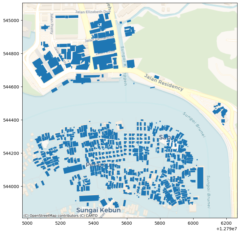
Cool, we see that there are some building are on water as expected 😁.

1️⃣ Pair image chips with bounding boxes 🧑‍🤝‍🧑

Here comes the fun 🛝 part! This section is all about generating 128x128 chips 🫶 paired with bounding boxes. Let’s go 🚲!

Create 128x128 raster chips and clip vector geometries with it ✂️

From the large 1280x1280 scene 🖽️, we will first slice out a hundred 128x128 chips 🍕 using zen3geo.datapipes.XbatcherSlicer (functional name: slice_with_xbatcher).

dp_raster = torchdata.datapipes.iter.IterableWrapper(iterable=[dataarray])
dp_xbatcher = dp_raster.slice_with_xbatcher(input_dims={"y": 128, "x": 128})
dp_xbatcher

XbatcherSlicerIterDataPipe

For each 128x128 chip 🍕, we’ll then find the vector geometries 🌙 that fit within the chip’s spatial extent. This will be 🤸 done using zen3geo.datapipes.GeoPandasRectangleClipper (functional name: clip_vector_with_rectangle).

dp_vector = torchdata.datapipes.iter.IterableWrapper(iterable=[gdf_kpgayer])
dp_clipped = dp_vector.clip_vector_with_rectangle(mask_datapipe=dp_xbatcher)
dp_clipped

GeoPandasRectangleClipperIterDataPipe

Important

When using zen3geo.datapipes.GeoPandasRectangleClipper 💇, there should only be one ‘global’ 🌐 vector geopandas.GeoSeries or geopandas.GeoDataFrame.

If your raster DataPipe has chips 🍕 with different coordinate reference systems (e.g. multiple UTM Zones 🌏🌍🌎), zen3geo.datapipes.GeoPandasRectangleClipper will actually reproject 🔄 the ‘global’ vector to the coordinate reference system of each chip, and clip ✂️ the geometries accordingly to the chip’s bounding box extent 😎.

This dp_clipped DataPipe will yield 🤲 a tuple of (vector, raster) objects for each 128x128 chip. Let’s inspect 🧐 one to see how they look like.

# Get one chip with over 10 building footprint geometries
for vector, raster in dp_clipped:
    if len(vector) > 10:
        break

These are the spatially subsetted vector geometries 🌙 in one 128x128 chip.

vector

	geometry	meanHeight
46097	POLYGON ((12795226.452 544733.061, 12795252.42...	-1.0
45521	POLYGON ((12795099.435 544690.503, 12795099.43...	-1.0
7770	POLYGON ((12795099.435 544773.939, 12795099.43...	-1.0
41199	POLYGON ((12795173.325 544771.647, 12795187.78...	-1.0
22585	POLYGON ((12795185.931 544790.568, 12795210.50...	-1.0
59109	POLYGON ((12795149.028 544777.963, 12795147.26...	-1.0
25608	POLYGON ((12795203.830 544826.201, 12795204.11...	-1.0
61424	POLYGON ((12795249.180 544754.879, 12795244.13...	-1.0
52194	POLYGON ((12795237.069 544763.752, 12795237.50...	-1.0
18183	POLYGON ((12795239.495 544843.496, 12795252.42...	-1.0
18302	POLYGON ((12795099.435 544814.744, 12795099.43...	-1.0
7350	POLYGON ((12795178.138 544843.496, 12795192.76...	-1.0
5108	POLYGON ((12795193.512 544843.496, 12795238.29...	-1.0

This is the raster chip/mask 🤿 used to clip the vector.

raster

<xarray.DataArray (band: 3, y: 128, x: 128)>
array([[[161, 141, 146, ..., 182, 188, 188],
        [148, 135, 128, ..., 182, 181, 184],
        [141, 118, 100, ..., 205, 201, 194],
        ...,
        [159, 160, 161, ...,  99,  93,  90],
        [162, 163, 164, ..., 113, 106,  83],
        [165, 165, 166, ..., 131, 117,  72]],

       [[150, 130, 135, ..., 169, 173, 173],
        [137, 124, 117, ..., 169, 168, 171],
        [132, 109,  91, ..., 194, 188, 181],
        ...,
        [148, 149, 150, ...,  88,  82,  79],
        [151, 152, 153, ..., 102,  95,  72],
        [154, 154, 155, ..., 120, 106,  61]],

       [[156, 136, 141, ..., 152, 154, 154],
        [143, 130, 121, ..., 152, 149, 152],
        [135, 112,  92, ..., 176, 171, 164],
        ...,
        [146, 147, 148, ...,  82,  76,  73],
        [149, 150, 151, ...,  98,  91,  68],
        [152, 152, 153, ..., 116, 104,  59]]], dtype=uint8)
Coordinates:
  * band         (band) int64 0 1 2
  * y            (y) float64 5.448e+05 5.448e+05 ... 5.447e+05 5.447e+05
  * x            (x) float64 1.28e+07 1.28e+07 1.28e+07 ... 1.28e+07 1.28e+07
    spatial_ref  int64 0

xarray.DataArray

• band: 3
• y: 128
• x: 128

• 161 141 146 144 159 151 157 143 136 ... 112 119 56 53 70 85 116 104 59

  array([[[161, 141, 146, ..., 182, 188, 188],
          [148, 135, 128, ..., 182, 181, 184],
          [141, 118, 100, ..., 205, 201, 194],
          ...,
          [159, 160, 161, ...,  99,  93,  90],
          [162, 163, 164, ..., 113, 106,  83],
          [165, 165, 166, ..., 131, 117,  72]],
  
         [[150, 130, 135, ..., 169, 173, 173],
          [137, 124, 117, ..., 169, 168, 171],
          [132, 109,  91, ..., 194, 188, 181],
          ...,
          [148, 149, 150, ...,  88,  82,  79],
          [151, 152, 153, ..., 102,  95,  72],
          [154, 154, 155, ..., 120, 106,  61]],
  
         [[156, 136, 141, ..., 152, 154, 154],
          [143, 130, 121, ..., 152, 149, 152],
          [135, 112,  92, ..., 176, 171, 164],
          ...,
          [146, 147, 148, ...,  82,  76,  73],
          [149, 150, 151, ...,  98,  91,  68],
          [152, 152, 153, ..., 116, 104,  59]]], dtype=uint8)

• Coordinates: (4)
  • band
    (band)
    int64
    0 1 2

    array([0, 1, 2])

  • y
    (y)
    float64
    5.448e+05 5.448e+05 ... 5.447e+05

    array([544842.898564, 544841.703302, 544840.50804 , 544839.312777,
           544838.117515, 544836.922252, 544835.72699 , 544834.531728,
           544833.336465, 544832.141203, 544830.945941, 544829.750678,
           544828.555416, 544827.360154, 544826.164891, 544824.969629,
           544823.774366, 544822.579104, 544821.383842, 544820.188579,
           544818.993317, 544817.798055, 544816.602792, 544815.40753 ,
           544814.212267, 544813.017005, 544811.821743, 544810.62648 ,
           544809.431218, 544808.235956, 544807.040693, 544805.845431,
           544804.650169, 544803.454906, 544802.259644, 544801.064381,
           544799.869119, 544798.673857, 544797.478594, 544796.283332,
           544795.08807 , 544793.892807, 544792.697545, 544791.502283,
           544790.30702 , 544789.111758, 544787.916495, 544786.721233,
           544785.525971, 544784.330708, 544783.135446, 544781.940184,
           544780.744921, 544779.549659, 544778.354397, 544777.159134,
           544775.963872, 544774.768609, 544773.573347, 544772.378085,
           544771.182822, 544769.98756 , 544768.792298, 544767.597035,
           544766.401773, 544765.20651 , 544764.011248, 544762.815986,
           544761.620723, 544760.425461, 544759.230199, 544758.034936,
           544756.839674, 544755.644412, 544754.449149, 544753.253887,
           544752.058624, 544750.863362, 544749.6681  , 544748.472837,
           544747.277575, 544746.082313, 544744.88705 , 544743.691788,
           544742.496526, 544741.301263, 544740.106001, 544738.910738,
           544737.715476, 544736.520214, 544735.324951, 544734.129689,
           544732.934427, 544731.739164, 544730.543902, 544729.34864 ,
           544728.153377, 544726.958115, 544725.762852, 544724.56759 ,
           544723.372328, 544722.177065, 544720.981803, 544719.786541,
           544718.591278, 544717.396016, 544716.200754, 544715.005491,
           544713.810229, 544712.614966, 544711.419704, 544710.224442,
           544709.029179, 544707.833917, 544706.638655, 544705.443392,
           544704.24813 , 544703.052867, 544701.857605, 544700.662343,
           544699.46708 , 544698.271818, 544697.076556, 544695.881293,
           544694.686031, 544693.490769, 544692.295506, 544691.100244])

  • x
    (x)
    float64
    1.28e+07 1.28e+07 ... 1.28e+07

    array([12795100.032295, 12795101.227557, 12795102.42282 , 12795103.618082,
           12795104.813344, 12795106.008607, 12795107.203869, 12795108.399132,
           12795109.594394, 12795110.789656, 12795111.984919, 12795113.180181,
           12795114.375443, 12795115.570706, 12795116.765968, 12795117.961231,
           12795119.156493, 12795120.351755, 12795121.547018, 12795122.74228 ,
           12795123.937542, 12795125.132805, 12795126.328067, 12795127.523329,
           12795128.718592, 12795129.913854, 12795131.109117, 12795132.304379,
           12795133.499641, 12795134.694904, 12795135.890166, 12795137.085428,
           12795138.280691, 12795139.475953, 12795140.671215, 12795141.866478,
           12795143.06174 , 12795144.257003, 12795145.452265, 12795146.647527,
           12795147.84279 , 12795149.038052, 12795150.233314, 12795151.428577,
           12795152.623839, 12795153.819101, 12795155.014364, 12795156.209626,
           12795157.404889, 12795158.600151, 12795159.795413, 12795160.990676,
           12795162.185938, 12795163.3812  , 12795164.576463, 12795165.771725,
           12795166.966988, 12795168.16225 , 12795169.357512, 12795170.552775,
           12795171.748037, 12795172.943299, 12795174.138562, 12795175.333824,
           12795176.529086, 12795177.724349, 12795178.919611, 12795180.114874,
           12795181.310136, 12795182.505398, 12795183.700661, 12795184.895923,
           12795186.091185, 12795187.286448, 12795188.48171 , 12795189.676972,
           12795190.872235, 12795192.067497, 12795193.26276 , 12795194.458022,
           12795195.653284, 12795196.848547, 12795198.043809, 12795199.239071,
           12795200.434334, 12795201.629596, 12795202.824858, 12795204.020121,
           12795205.215383, 12795206.410646, 12795207.605908, 12795208.80117 ,
           12795209.996433, 12795211.191695, 12795212.386957, 12795213.58222 ,
           12795214.777482, 12795215.972745, 12795217.168007, 12795218.363269,
           12795219.558532, 12795220.753794, 12795221.949056, 12795223.144319,
           12795224.339581, 12795225.534843, 12795226.730106, 12795227.925368,
           12795229.120631, 12795230.315893, 12795231.511155, 12795232.706418,
           12795233.90168 , 12795235.096942, 12795236.292205, 12795237.487467,
           12795238.682729, 12795239.877992, 12795241.073254, 12795242.268517,
           12795243.463779, 12795244.659041, 12795245.854304, 12795247.049566,
           12795248.244828, 12795249.440091, 12795250.635353, 12795251.830615])

  • spatial_ref
    ()
    int64
    0

    crs_wkt :

    PROJCS["WGS 84 / Pseudo-Mercator",GEOGCS["WGS 84",DATUM["WGS_1984",SPHEROID["WGS 84",6378137,298.257223563,AUTHORITY["EPSG","7030"]],AUTHORITY["EPSG","6326"]],PRIMEM["Greenwich",0,AUTHORITY["EPSG","8901"]],UNIT["degree",0.0174532925199433,AUTHORITY["EPSG","9122"]],AUTHORITY["EPSG","4326"]],PROJECTION["Mercator_1SP"],PARAMETER["central_meridian",0],PARAMETER["scale_factor",1],PARAMETER["false_easting",0],PARAMETER["false_northing",0],UNIT["metre",1,AUTHORITY["EPSG","9001"]],AXIS["Easting",EAST],AXIS["Northing",NORTH],EXTENSION["PROJ4","+proj=merc +a=6378137 +b=6378137 +lat_ts=0 +lon_0=0 +x_0=0 +y_0=0 +k=1 +units=m +nadgrids=@null +wktext +no_defs"],AUTHORITY["EPSG","3857"]]

    spatial_ref :

    PROJCS["WGS 84 / Pseudo-Mercator",GEOGCS["WGS 84",DATUM["WGS_1984",SPHEROID["WGS 84",6378137,298.257223563,AUTHORITY["EPSG","7030"]],AUTHORITY["EPSG","6326"]],PRIMEM["Greenwich",0,AUTHORITY["EPSG","8901"]],UNIT["degree",0.0174532925199433,AUTHORITY["EPSG","9122"]],AUTHORITY["EPSG","4326"]],PROJECTION["Mercator_1SP"],PARAMETER["central_meridian",0],PARAMETER["scale_factor",1],PARAMETER["false_easting",0],PARAMETER["false_northing",0],UNIT["metre",1,AUTHORITY["EPSG","9001"]],AXIS["Easting",EAST],AXIS["Northing",NORTH],EXTENSION["PROJ4","+proj=merc +a=6378137 +b=6378137 +lat_ts=0 +lon_0=0 +x_0=0 +y_0=0 +k=1 +units=m +nadgrids=@null +wktext +no_defs"],AUTHORITY["EPSG","3857"]]

    array(0)

• Indexes: (3)
  • band
    PandasIndex

    PandasIndex(Index([0, 1, 2], dtype='int64', name='band'))

  • y
    PandasIndex

    PandasIndex(Index([544842.8985642623, 544841.7033018966,  544840.508039531,
           544839.3127771653, 544838.1175147996,  544836.922252434,
           544835.7269900682, 544834.5317277026, 544833.3364653368,
           544832.1412029712,
           ...
           544701.8576051121, 544700.6623427465, 544699.4670803808,
           544698.2718180151, 544697.0765556494, 544695.8812932838,
            544694.686030918, 544693.4907685524, 544692.2955061867,
            544691.100243821],
          dtype='float64', name='y', length=128))

  • x
    PandasIndex

    PandasIndex(Index([12795100.032295031, 12795101.227557397, 12795102.422819762,
           12795103.618082128, 12795104.813344494, 12795106.008606859,
           12795107.203869225,  12795108.39913159, 12795109.594393956,
           12795110.789656322,
           ...
           12795241.073254181, 12795242.268516546, 12795243.463778911,
           12795244.659041278, 12795245.854303643, 12795247.049566008,
           12795248.244828375,  12795249.44009074, 12795250.635353105,
           12795251.830615472],
          dtype='float64', name='x', length=128))

• Attributes: (0)

And here’s a side by side visualization of the 🌈 RGB chip image (left) and 🔷 vector building footprint polygons (right).

fig, ax = plt.subplots(ncols=2, figsize=(18, 9), sharex=True, sharey=True)
raster.plot.imshow(ax=ax[0])
vector.plot(ax=ax[1])

<Axes: >

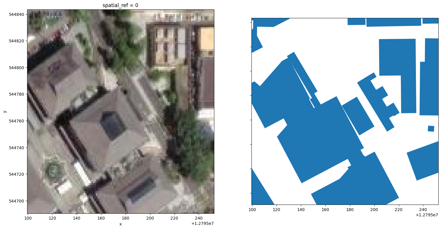
Cool, these buildings are part of the 🏬 Yayasan Shopping Complex in Bandar Seri Begawan 🌆. We can see that the raster image 🖼️ on the left aligns ok with the vector polygons 💠 on the right.

Note

The optical 🛰️ imagery shown here is not the imagery used to digitize the building footprints 🏢! This is an example tutorial using two different data sources, that we just so happened to have plotted in the same geographic space 😝.

From polygons in geographic coordinates to boxes in image coordinates ↕️

Up to this point, we still have the actual 🛖 building footprint polygons. In this step 📶, we’ll convert these polygons into a format suitable for ‘basic’ object detection 🥅 models in computer vision. Specifically:

1. The polygons 🌙 (with multiple vertices) will be simplified to a horizontal bounding box 🔲 with 4 corner vertices only.

2. The 🌐 geographic coordinates of the box which use lower left corner and upper right corner (i.e. y increases from South to North ⬆️) will be converted to 🖼️ image coordinates (0-128) which use the top left corner and bottom right corner (i.e y increases from Top to Bottom ⬇️).

Let’s start by using geopandas.GeoSeries.bounds to get the geographic bounds 🗺️ of each building footprint geometry 📐 in each 128x128 chip.

def polygon_to_bbox(geom_and_chip) -> (gpd.GeoDataFrame, xr.DataArray):
    """
    Get bounding box (minx, miny, maxx, maxy) coordinates for each geometry in
    a geopandas.GeoDataFrame.

                          (maxx,maxy)
               ul-------ur
             ^  |       |
             |  |  geo  |    y increases going up, x increases going right
             y  |       |
               ll-------lr
    (minx,miny)    x-->

    """
    gdf, chip = geom_and_chip
    bounds: gpd.GeoDataFrame = gdf.bounds
    assert tuple(bounds.columns) == ("minx", "miny", "maxx", "maxy")

    return bounds, chip

dp_bbox = dp_clipped.map(fn=polygon_to_bbox)

Next, the geographic 🗺️ bounding box coordinates (in EPSG:3857) will be converted to image 🖼️ or pixel coordinates (0-128 scale). The y-direction will be flipped 🤸 upside down, and we’ll be using the spatial bounds (or corner coordinates) of the 128x128 image chip as a reference 📍.

def geobox_to_imgbox(bbox_and_chip) -> (pd.DataFrame, xr.DataArray):
    """
    Convert bounding boxes in a pandas.DataFrame from geographic coordinates
    (minx, miny, maxx, maxy) to image coordinates (x1, y1, x2, y2) based on the
    spatial extent of a raster image chip.

        (x1,y1)
               ul-------ur
             y  |       |
             |  |  img  |    y increases going down, x increases going right
             v  |       |
               ll-------lr
                   x-->    (x2,y2)

    """
    geobox, chip = bbox_and_chip

    x_res, y_res = chip.rio.resolution()
    assert y_res < 0

    left, bottom, right, top = chip.rio.bounds()
    assert top > bottom

    imgbox = pd.DataFrame()
    imgbox["x1"] = (geobox.minx - left) / x_res  # left
    imgbox["y1"] = (top - geobox.maxy) / -y_res  # top
    imgbox["x2"] = (geobox.maxx - left) / x_res  # right
    imgbox["y2"] = (top - geobox.miny) / -y_res  # bottom

    assert all(imgbox.x2 > imgbox.x1)
    assert all(imgbox.y2 > imgbox.y1)

    return imgbox, chip

dp_ibox = dp_bbox.map(fn=geobox_to_imgbox)

Now to plot 🎨 and double check that the boxes are positioned correctly in 0-128 image space 🌌.

# Get one chip with over 10 building footprint geometries
for ibox, ichip in dp_ibox:
    if len(ibox) > 10:
        break
ibox

	x1	y1	x2	y2
46097	106.267600	84.477237	128.000000	111.487401
45521	0.000000	102.624007	15.915053	128.000000
7770	0.000000	27.158230	101.079502	128.000000
41199	61.819662	53.976790	84.270007	80.526231
22585	72.365741	37.279512	101.486711	77.930713
59109	24.359445	23.205062	47.607712	61.791212
25608	87.341014	14.232860	112.921057	65.286400
61424	120.748550	73.796988	125.282081	78.005132
52194	115.149687	13.901857	128.000000	66.843693
18183	117.179471	0.000000	128.000000	3.929291
18302	0.000000	0.000000	26.325074	24.055215
7350	65.845721	0.000000	78.135024	4.845090
5108	78.708163	0.000000	116.277647	5.983405

fig, ax = plt.subplots(ncols=2, figsize=(18, 9), sharex=True, sharey=True)
ax[0].imshow(X=ichip.transpose("y", "x", "band"))
for i, row in ibox.iterrows():
    rectangle = matplotlib.patches.Rectangle(
        xy=(row.x1, row.y1),
        width=row.x2 - row.x1,
        height=row.y2 - row.y1,
        edgecolor="blue",
        linewidth=1,
        facecolor="none",
    )
    ax[1].add_patch(rectangle)

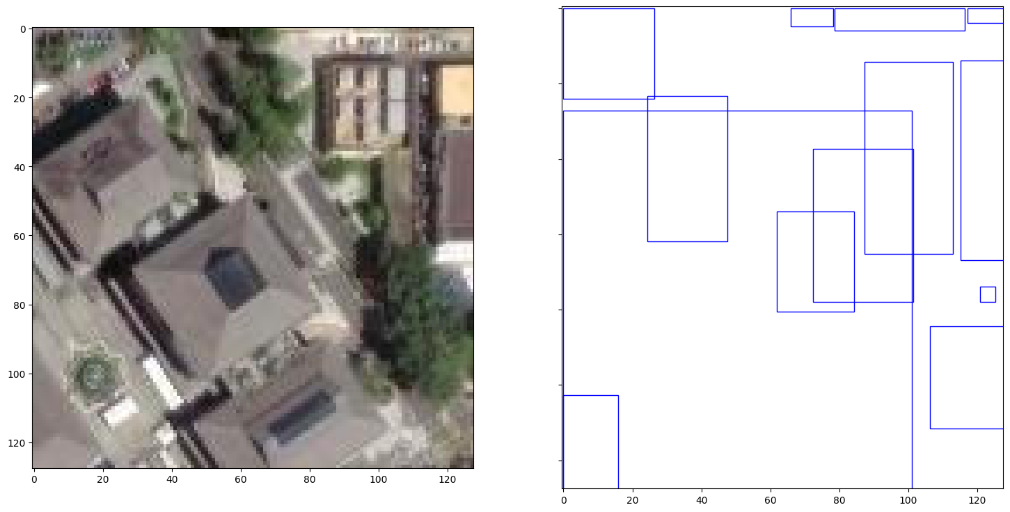
Cool, the 🟦 bounding boxes on the right subplot are correctly positioned 🧭 (compare it with the figure in the previous subsection).

Hint

Instead of a bounding box 🥡 object detection task, you can also use the building polygons 🏘️ for a segmentation task 🧑‍🎨 following Vector segmentation masks.

If you still prefer doing object detection 🕵️, but want a different box format (see options in torchvision.ops.box_convert()), like 🎌 centre-based coordinates with width and height (cxcywh), or 📨 oriented/rotated bounding box coordinates, feel free to implement your own function and DataPipe for it 🤗!

2️⃣ There and back again 🧙

What follows on from here requires focus 🤫. To start, we’ll pool the hundred 💯 128x128 chips into 10 batches (10 chips per batch) using torchdata.datapipes.iter.Batcher (functional name: batch).

dp_batch = dp_ibox.batch(batch_size=10)
print(f"Number of items in first batch: {len(list(dp_batch)[0])}")

Number of items in first batch: 10

Batch boxes with variable lengths 📏

Next, we’ll stack 🥞 all the image chips into a single tensor (recall Chipping and batching data), and concatenate 📚 the bounding boxes into a list of tensors using torchdata.datapipes.iter.Collator (functional name: collate).

def boximg_collate_fn(samples) -> (list[torch.Tensor], torch.Tensor, list[dict]):
    """
    Converts bounding boxes and raster images to tensor objects and keeps
    geographic metadata (spatial extent, coordinate reference system and
    spatial resolution).

    Specifically, the bounding boxes in pandas.DataFrame format are each
    converted to a torch.Tensor and collated into a list, while the raster
    images in xarray.DataArray format are converted to a torch.Tensor (int16
    dtype) and stacked into a single torch.Tensor.
    """
    box_tensors: list[torch.Tensor] = [
        torch.as_tensor(sample[0].to_numpy(dtype=np.float32)) for sample in samples
    ]

    tensors: list[torch.Tensor] = [
        torch.as_tensor(data=sample[1].data.astype(dtype="int16")) for sample in samples
    ]
    img_tensors = torch.stack(tensors=tensors)

    metadata: list[dict] = [
        {
            "bbox": sample[1].rio.bounds(),
            "crs": sample[1].rio.crs,
            "resolution": sample[1].rio.resolution(),
        }
        for sample in samples
    ]

    return box_tensors, img_tensors, metadata

dp_collate = dp_batch.collate(collate_fn=boximg_collate_fn)
print(f"Number of mini-batches: {len(dp_collate)}")
mini_batch_box, mini_batch_img, mini_batch_metadata = list(dp_collate)[1]
print(f"Mini-batch image tensor shape: {mini_batch_img.shape}")
print(f"Mini-batch box tensors: {mini_batch_box}")
print(f"Mini-batch metadata: {mini_batch_metadata}")

Number of mini-batches: 10

Mini-batch image tensor shape: torch.Size([10, 3, 128, 128])
Mini-batch box tensors: [tensor([[123.9093, 104.9202, 128.0000, 128.0000],
        [112.9828, 106.5683, 118.8773, 124.6974],
        [113.1629,  26.8098, 128.0000,  44.9749]]), tensor([[117.0043, 115.3977, 128.0000, 128.0000],
        [  0.0000, 104.9909,  26.1012, 128.0000],
        [ 65.7458, 118.2312,  78.0862, 128.0000],
        [ 78.5054, 116.4489, 116.1789, 128.0000],
        [  3.0884,  47.5740,   9.3976,  52.5646],
        [  0.0000,  18.7743,  28.4082,  45.3366]]), tensor([[117.9412, 100.7308, 128.0000, 128.0000],
        [115.7629,  74.4706, 124.1512,  83.4432],
        [ 36.1700, 119.8452,  74.3699, 128.0000],
        [  0.0000, 115.3069,  35.1435, 128.0000],
        [110.2586,  65.3755, 128.0000,  91.0184],
        [111.3105,  69.6327, 118.5406,  75.7000],
        [101.3318,   3.0389, 128.0000,  67.6447]]), tensor([[  0.0000,  87.2009, 106.9465, 128.0000],
        [ 53.5764,  47.6009,  98.3723,  81.2635],
        [126.2443,   4.6490, 128.0000,  14.6764],
        [  0.0000,  63.6644,  16.4110,  88.8571],
        [ 15.2246,  58.3821,  56.9873,  88.2886],
        [ 22.5505,  26.3118,  33.0069,  35.9500],
        [ 13.6754,  25.8521,  21.1058,  32.7201],
        [ 18.9505,  15.9668,  27.8914,  24.1055],
        [  0.0000,   0.0000,  90.5514,  61.9928]]), tensor([[ 0.0000,  4.4358,  9.4605, 14.6412],
        [21.1518, 26.8578, 74.4305, 80.4817],
        [21.9534, 43.8958, 55.8650, 59.0243],
        [72.5806, 47.9954, 77.5368, 53.9594],
        [22.3033, 45.0466, 28.6352, 49.5979],
        [45.8440, 40.1061, 51.2531, 44.5580],
        [34.4906,  0.0000, 55.9927,  9.6874]]), tensor([], size=(0, 4)), tensor([], size=(0, 4)), tensor([], size=(0, 4)), tensor([], size=(0, 4)), tensor([], size=(0, 4))]
Mini-batch metadata: [{'bbox': (12794946.441081041, 544843.4961954451, 12795099.434663847, 544996.4897782521), 'crs': CRS.from_epsg(3857), 'resolution': (1.1952623656738226, -1.1952623656793226)}, {'bbox': (12795099.434663849, 544843.4961954451, 12795252.428246655, 544996.4897782521), 'crs': CRS.from_epsg(3857), 'resolution': (1.1952623656738226, -1.1952623656793226)}, {'bbox': (12795252.428246655, 544843.4961954451, 12795405.42182946, 544996.4897782521), 'crs': CRS.from_epsg(3857), 'resolution': (1.1952623656738226, -1.1952623656793226)}, {'bbox': (12795405.421829462, 544843.4961954451, 12795558.415412268, 544996.4897782521), 'crs': CRS.from_epsg(3857), 'resolution': (1.1952623656738226, -1.1952623656793226)}, {'bbox': (12795558.415412268, 544843.4961954451, 12795711.408995073, 544996.4897782521), 'crs': CRS.from_epsg(3857), 'resolution': (1.1952623656738226, -1.1952623656793226)}, {'bbox': (12795711.408995075, 544843.4961954451, 12795864.40257788, 544996.4897782521), 'crs': CRS.from_epsg(3857), 'resolution': (1.1952623656738226, -1.1952623656793226)}, {'bbox': (12795864.40257788, 544843.4961954451, 12796017.396160686, 544996.4897782521), 'crs': CRS.from_epsg(3857), 'resolution': (1.1952623656738226, -1.1952623656793226)}, {'bbox': (12796017.396160688, 544843.4961954451, 12796170.389743494, 544996.4897782521), 'crs': CRS.from_epsg(3857), 'resolution': (1.1952623656738226, -1.1952623656793226)}, {'bbox': (12796170.389743494, 544843.4961954451, 12796323.3833263, 544996.4897782521), 'crs': CRS.from_epsg(3857), 'resolution': (1.1952623656738226, -1.1952623656793226)}, {'bbox': (12796323.383326301, 544843.4961954451, 12796476.376909107, 544996.4897782521), 'crs': CRS.from_epsg(3857), 'resolution': (1.1952623656738226, -1.1952623656793226)}]

The DataPipe is complete 🙌, let’s visualize the entire data pipeline graph.

torchdata.datapipes.utils.to_graph(dp=dp_collate)

Into a DataLoader 🏋️

Loop over the DataPipe using torch.utils.data.DataLoader ⚙️!

dataloader = torchdata.dataloader2.DataLoader2(datapipe=dp_collate)
for i, batch in enumerate(dataloader):
    box, img, metadata = batch
    print(f"Batch {i} - img: {img.shape}, box sizes: {[len(b) for b in box]}")

Batch 0 - img: torch.Size([10, 3, 128, 128]), box sizes: [0, 3, 1, 2, 1, 0, 0, 0, 0, 0]
Batch 1 - img: torch.Size([10, 3, 128, 128]), box sizes: [3, 6, 7, 9, 7, 0, 0, 0, 0, 0]
Batch 2 - img: torch.Size([10, 3, 128, 128]), box sizes: [3, 13, 8, 4, 1, 0, 0, 0, 0, 0]

Batch 3 - img: torch.Size([10, 3, 128, 128]), box sizes: [1, 4, 3, 4, 2, 2, 0, 0, 0, 0]
Batch 4 - img: torch.Size([10, 3, 128, 128]), box sizes: [0, 0, 1, 1, 4, 2, 0, 8, 3, 0]

Batch 5 - img: torch.Size([10, 3, 128, 128]), box sizes: [5, 27, 37, 43, 36, 38, 18, 1, 2, 0]
Batch 6 - img: torch.Size([10, 3, 128, 128]), box sizes: [15, 40, 28, 56, 32, 31, 36, 4, 0, 0]

Batch 7 - img: torch.Size([10, 3, 128, 128]), box sizes: [3, 3, 24, 33, 45, 49, 44, 2, 0, 0]
Batch 8 - img: torch.Size([10, 3, 128, 128]), box sizes: [0, 0, 3, 6, 1, 9, 14, 1, 0, 0]
Batch 9 - img: torch.Size([10, 3, 128, 128]), box sizes: [0, 0, 0, 0, 0, 0, 0, 0, 0, 0]

There’s probably hundreds of models you can 🍜 feed this data into, from mmdetection’s 模型库 🐼 to torchvision’s Models and pre-trained weights). But are we out of the woods yet?

Georeference image boxes 📍

To turn the model’s predicted bounding boxes in image space 🌌 back to geographic coordinates 🌐, you’ll need to use an affine transform. Assuming you’ve kept your 🏷️ metadata intact, here’s an example on how to do the georeferencing:

for batch in dataloader:
    pred_boxes, images, metadata = batch

    objs: list = []
    for idx in range(0, len(images)):
        left, bottom, right, top = metadata[idx]["bbox"]
        crs = metadata[idx]["crs"]
        x_res, y_res = metadata[idx]["resolution"]

        gdf = gpd.GeoDataFrame(
            geometry=[
                shapely.affinity.affine_transform(
                    geom=shapely.geometry.box(*coords),
                    matrix=[x_res, 0, 0, y_res, left, top],
                )
                for coords in pred_boxes[idx]
            ],
            crs=crs,
        )
        objs.append(gdf.to_crs(crs=crs))

    geodataframe: gpd.GeoDataFrame = pd.concat(objs=objs, ignore_index=True)
    geodataframe.set_crs(crs=crs, inplace=True)
    break

geodataframe

	geometry
0	POLYGON ((12795245.323 545027.959, 12795245.32...
1	POLYGON ((12795252.428 545028.185, 12795252.42...
2	POLYGON ((12795227.218 545027.685, 12795227.21...
3	POLYGON ((12795306.384 545029.400, 12795306.38...
4	POLYGON ((12795496.658 545045.087, 12795496.65...
5	POLYGON ((12795504.103 545037.782, 12795504.10...
6	POLYGON ((12795623.979 545002.809, 12795623.97...

Back at square one, or are we?